The essence of a select query is to select rows from the source table that meet certain criteria (similar to using a standard one). Let's select values from the source table using. Unlike using ( CTRL + SHIFT + L or Data / Sort and Filter / Filter) the selected rows will be placed in a separate table.
In this article, we will consider the most common queries, for example: selection of table rows whose value from a numeric column falls within a specified range (interval); selection of rows for which the date is a certain period; tasks with 2 text criteria and others. Let's start with simple queries.
1. One numerical criterion (Select those Products for which the price is higher than the minimum)
example file, sheet One criterion is number ).
It is necessary to display in a separate table only those records (rows) from the Source table for which the price is higher than 25.
You can easily solve this and subsequent tasks with the help of. To do this, select the headers of the Source table and press CTRL + SHIFT + L... Using the drop-down list at the heading Prices select Number Filters ..., then set the required filtering conditions and click OK.

Records matching the selection criteria will be displayed.

Another approach is to use. In contrast to the selected rows, they will be placed in a separate table - a kind, which, for example, can be formatted in a style different from the Source table or make its other modifications.
Place the criterion (minimum price) in the cell E6 , table for filtered data - in the range D10: E19 .

Now let's select the range D11: D19 (column Product) and enter:
INDEX (A11: A19;
SMALL (IF ($ E $ 6<=B11:B19;СТРОКА(B11:B19);"");СТРОКА()-СТРОКА($B$10))
-LINE ($ B $ 10))
Instead of ENTER press the keyboard shortcut CTRL + SHIFT + ENTER(array formula will be).
E11: E19 (column Price) where we will enter a similar one:
INDEX (B11: B19;
SMALL (IF ($ E $ 6<=B11:B19;СТРОКА(B11:B19);"");СТРОКА()-СТРОКА($B$10))
-LINE ($ B $ 10))
As a result, we will get a new table that will contain only products with prices not less than the one specified in the cell E6 .
To show the dynamism of the received Sample Request, we introduce into E6 value 55. Only 2 records will get into the new table.

If you add a new product with a Price of 80 to the Source table, a new record will be automatically added to the new table.

Note... You can also use and to display filtered data. The choice of a specific tool depends on the task facing the user.
If you are not comfortable using array formula, which returns multiple values, you can use a different approach, which is discussed in the sections below: 5.a, 7, 10, and 11. In these cases, are used.
2. Two numerical criteria (Select those Products for which the price falls within the range)
Let there be an Initial table with a list of Products and Prices (see. example file, sheetRange of Numbers).
Place the criteria (lower and upper price boundaries) in the range E5: E6 .

Those. if the Price of the Goods falls within the specified interval, then such a record will appear in the new Filtered data table.
Unlike the previous task, we will create two: Products and Prices (you can do without them, but they are convenient when writing formulas). The corresponding formulas should look in the Name Manager ( Formulas / Defined Names / Name Manager) as follows (see figure below).

Now let's select the range D11: D19 and in we introduce:
INDEX (Goods;
LEAST(
IF (($ E $ 5<=Цены)*($E$6>= Prices); LINE (Prices); "");
Instead of ENTER press the keyboard shortcut CTRL + SHIFT + ENTER.
We will perform the same manipulations with the range E11: E19 where we will introduce a similar one:
INDEX (Prices;
LEAST(
IF (($ E $ 5<=Цены)*($E$6>= Prices); LINE (Prices); "");
LINE (Prices) -LINE ($ B $ 10)) - LINE ($ B $ 10))
As a result, we will get a new table that will contain only products for which prices fall within the interval specified in the cells E5 and E6 .

To show the dynamism of the received Report (Request for selection), we enter in E6 value 65. One more record from the Source table will be added to the new table, satisfying the new criterion.

If you add a new product with a Price in the range from 25 to 65 to the Source table, then a new record will be added to the new table.

The sample file also contains array formulas that handle errors when the Price column contains an error value, such as # DIV / 0! (see sheet Error processing).
The following tasks are solved in a similar way, so we will not consider them in detail.
3. One criterion Date (Select those Products for which the Delivery Date matches the specified one)
example file, sheetOne criterion - Date).

To select rows, array formulas are used, similar to Task1 (instead of the criterion<= используется =):
=INDEX (A12: A20; SMALL (IF ($ E $ 6 = B12: B20; LINE (B12: B20); ""); LINE (B12: B20) -LINE ($ B $ 11)) - LINE ($ B $ 11) )
INDEX (B12: B20; SMALL (IF ($ E $ 6 = B12: B20; LINE (B12: B20); ""); LINE (B12: B20) -LINE ($ B $ 11)) - LINE ($ B $ 11) )
4. Two criteria Date (Select those Products for which the Delivery Date falls within the range)
Suppose there is an Initial table with a list of Goods and Delivery dates (see. example file, sheetDate range).

Note that the Date column is NOT SORTED.
Solution1: You can use to filter rows.
Enter into cell D12 array formula:
INDEX (A $ 12: A $ 20;
LARGE (($ E $ 6<=$B$12:$B$20)*($E$7>= $ B $ 12: $ B $ 20) * (LINE ($ B $ 12: $ B $ 20) -LINE ($ B $ 11));
$ J $ 12-LINE (A12) + LINE ($ B $ 11) +1))
Note: After entering the formula, instead of the ENTER key, press the CTRL + SHIFT + ENTER key combination. This keyboard shortcut is used to enter array formulas.
Copy the array formula down to the desired number of cells. The formula will return only those values of Products that were delivered within the specified date range. The rest of the cells will contain #NUM! Errors. Errors in example file (Sheet 4 Date Range) .
A similar formula must be entered for the dates in column E.
In a cell J12 calculated the number of rows of the source table that meet the criteria:
COUNTIFS (B12: B20; "> =" & $ E $ 6; B12: B20; "<="&$E$7)
Source table rows that meet the criteria are.
Solution2: To select rows, you can use array formulas similar to Task2 (i.e.):
=INDEX (A12: A20; SMALL (IF (($ E $ 6<=B12:B20)*($E$7>= B12: B20); LINE (B12: B20); ""); LINE (B12: B20) -LINE ($ B $ 11)) - LINE ($ B $ 11))
INDEX (B12: B20; SMALL (IF (($ E $ 6<=B12:B20)*($E$7>= B12: B20); LINE (B12: B20); ""); LINE (B12: B20) -LINE ($ B $ 11)) - LINE ($ B $ 11))
To enter the first formula, select a range of cells G12: G20 ... After entering the formula, instead of the ENTER key, press the CTRL + SHIFT + ENTER key combination.
Solution3: If the Date column is SORTED, then you do not need to use array formulas.
First, you need to calculate the first and last positions of the rows that meet the criteria. Then print the lines.

This example once again clearly demonstrates how much easier it is to write formulas.
5. One criterion Date (Select those Goods for which the Delivery Date is not earlier / not later than the specified one)
Suppose there is an Initial table with a list of Goods and Delivery dates (see. example file, sheet One criterion - Date (no later than) ).

To select rows whose date is not earlier (including the date itself), use the array formula:
=INDEX (A12: A20; SMALL (IF ($ E $ 7<=B12:B20;СТРОКА(B12:B20);"");СТРОКА(B12:B20)-СТРОКА($B$11))-СТРОКА($B$11))
Also, the example file contains formulas for conditions: Not earlier (not including); No later (including); No later (not including).
7. One Text Criterion (Select Products of a certain type)
Let there be an Initial table with a list of Products and Prices (see. example file, sheetOne criterion - Text).

8. Two Text Criteria (Select Goods of a certain type delivered in a given month)
Let there be an Initial table with a list of Products and Prices (see. example file, sheet 2 criteria - text (I) ).

INDEX ($ A $ 11: $ A $ 19;
SMALL (IF (($ F $ 6 = $ A $ 11: $ A $ 19) * ($ F $ 7 = $ B $ 11: $ B $ 19); LINE ($ A $ 11: $ A $ 19) -LINE ($ A $ 10); 30); LINE (INDIRECT ("A1: A" & ROWS ($ A $ 11: $ A $ 19)))))
Expression ($ F $ 6 = $ A $ 11: $ A $ 19) * ($ F $ 7 = $ B $ 11: $ B $ 19) sets both conditions (Item and Month).
Expression LINE (INDIRECT ("A1: A" & ROWS ($ A $ 11: $ A $ 19))) forms (1: 2: 3: 4: 5: 6: 7: 8: 9), i.e. row numbers in the table.
9. Two Text Criteria (Select Products of Certain Types)
Let there be an Initial table with a list of Products and Prices (see. example file, sheet2 criteria - text (OR)).
Unlike Problem 7, select the rows with goods of 2 types ().

The array formula is used to select rows:
INDEX (A $ 11: A $ 19;
LARGE ((($ E $ 6 = $ A $ 11: $ A $ 19) + ($ E $ 7 = $ A $ 11: $ A $ 19)) * (ROW ($ A $ 11: $ A $ 19) -LINE ($ A $ 10) ); COUNTIF ($ A $ 11: $ A $ 19; $ E $ 6) + COUNTIF ($ A $ 11: $ A $ 19; $ E $ 7) -ROWS ($ A $ 11: A11) +1))
Condition ($ E $ 6 = $ A $ 11: $ A $ 19) + ($ E $ 7 = $ A $ 11: $ A $ 19) guarantees that only the specified types of goods will be selected from the yellow cells (Product2 and Product3). The + (addition) sign is used for the task (at least 1 criterion must be met).
The above expression will return an array (0: 0: 0: 0: 1: 1: 1: 0: 0). Multiplying it by the expression LINE ($ A $ 11: $ A $ 19) -LINE ($ A $ 10), i.e. on (1: 2: 3: 4: 5: 6: 7: 8: 9), we get an array of positions (table row numbers) that meet the criteria. In our case, it will be an array (0: 0: 0: 0: 5: 6: 7: 0: 0).
As an example, we present solutions to the following problem: Select Products, the price of which lies in a certain range and is repeated a specified number of times or more.
Let's take the table of consignments of goods as the initial one.

Suppose that we are interested in how many and what consignments of goods were supplied at a price of 1000 rubles. up to 2000r. (criterion 1). Moreover, there must be at least 3 parties with the same price (criterion 2).
The solution is an array formula:
SMALL (ROW ($ A $ 14: $ A $ 27) * ($ C $ 14: $ C $ 27> = $ B $ 7) * ($ C $ 14: $ C $ 27<=$C$7)*($D$14:$D$27>= $ B $ 10); F14 + ($ G $ 8- $ G $ 9))
This formula returns line numbers that meet both criteria.
Formula = SUMPRODUCT (($ C $ 14: $ C $ 27> = $ B $ 7) * ($ C $ 14: $ C $ 27<=$C$7)*($D$14:$D$27>= $ B $ 10)) counts the number of rows that meet the criteria.
11. We use the value of the criterion (Any) or (All)

V example file on sheet "11. Criterion Any or (All)" this variant of the criterion has been implemented.
The formula in this case must contain the IF () function. If the value (All) is selected, then the formula is used to display values without taking into account this criterion. If any other value is selected, then the criterion works in the usual way.

IF ($ C $ 8 = "(All)";
SMALL ((LINE ($ B $ 13: $ B $ 26) -LINE ($ B $ 12)) * ($ D $ 13: $ D $ 26> = $ D $ 8); F13 + ($ G $ 6- $ G $ 7));
SMALL ((LINE ($ B $ 13: $ B $ 26) -LINE ($ B $ 12)) * ($ D $ 13: $ D $ 26> = $ D $ 8) * ($ C $ 13: $ C $ 26 = $ C $ 8) ; F13 + ($ G $ 6- $ G $ 7)))
The rest of the formula is similar to those discussed above.
Fetching data
Create a report on the sample from Sheet 5 in the column "Qualitative performance, percent." (from Sheet 8, table 7)
In order to sample data, you must perform the following steps:
Determine the number of elements of a new array according to a given condition by entering a variable using the InputBox operator
Declare and redeclare a new array
Form a new array. To do this, you need to set the number of the first element of the new array u = 1. Then a cycle is executed, in which the selection condition is written according to the column "Qualitative performance, percent." If the result of the check is true, then the element of the analyzed array becomes an element of the new array.
Display new element on Sheet 8
Sub ReportSample ()
Sheets ("Sheet8"). Select
Dim A () As Variant
ReDim A (1 To n1, 1 To m)
VVOD "Sheet5", A, n1, m, 4
C = InputBox ("Enter a condition")
Sheets ("Sheet8"). Cells (5.11) = C
For i = 1 To n1
If A (i,
8) >
d = d + 1
Sheets ("Sheet8"). Cells (5,10) = d
Dim B () As Variant
ReDim B (1 To d, 1 To m)
For i = 1 To n1
If A (i,
8)> Sheets ("Sheet8"). Cells (5.11) Then
For j = 1 To m
B (u, j) = A (i, j)
u = u + 1
For i = 1 To d
For j = 1 To m
Sheets ("Sheet8"). Cells (i + 4, j) = B (i, j)
Fig. 6. Table data after fetch
Creating an automatic macro on a selection
We turn on the recording of the macro. Tools> Macro> Start Recording> OK. A square will appear where the stop recording button is. On Sheet5 (report), select the table without headers and totals, copy it to Sheet10 (autoselection). Select the table without headers and in the menu item, select Data> Filter> AutoFilter> select the condition> OK. We mark the column by which we will sort. We finish the work of the macro.
Sub Macro2Sample ()
"Macro2Setup Macro
Sheets ("Sheet5"). Select
Selection. Copy
Sheets ("Sheet9"). Select
ActiveSheet. Paste
Range ("H5: H17"). Select
Application. CutCopyMode = False
Selection. AutoFilter
ActiveSheet. Range ("$ H $ 5: $ H $ 17"). AutoFilter Field: = 1, Criteria1: = "> 80", _

Operator: = xlAnd
Range ("G22"). Select
Fig. 7. Table data after autoselection

Determining the maximum and minimum value
Determine the max and min values for the columns "Total", "Absolute performance, percent.", "Qualitative performance" (table 9, sheet 10)
To determine the max and min values, you need to do the following:
Set the reference variable, which will be the current minimum (maximum)
Each element of the population is compared one by one with the current minimum (maximum), and if this element does not satisfy the search conditions (in the case of a minimum, it is greater, and in the case of a maximum, less), then the reference value is replaced by the value of the compared element
After a complete scan of all elements in the variable of the current minimum (maximum), the actual minimum (maximum) is found
The value of the minimum (maximum) is displayed in the corresponding cells
Sub minmax ()
Dim A () As Variant
n1 = Sheets ("Sheet4"). Cells (5.12)
m = Sheets ("Sheet2"). Cells (5.12)
ReDim A (1 To n1, 1 To m)
VVOD "Sheet5", A, n1, m, 4
VIVOD "Sheet10", A, n1, m, 4
VVOD "Sheet10", A, n1, m, 4
For j = 3 To m
maxA = 0.00001
minA = 1,000,000
For i = 1 To n1
If A (i, j)> maxA Then
maxA = A (i, j)
If A (i, j)< minA Then
minA = A (i, j)
Sheets ("Sheet10"). Cells (i + 4 + 2, j) = maxA
Sheets ("Sheet10"). Cells (i + 4 + 3, j) = minA

A macro is a sequence of actions that has been recorded and saved for future reference. The saved macro can be played back by a special command. In other words, you can record your actions in a macro, save it, and then allow other users to replay the actions saved in the macro with a simple keystroke. This is especially useful when distributing PivotTable reports.
Let's say you want to give your customers the ability to group PivotTable reports by month, quarter, and year. Technically, the grouping process can be done by any user, but some of your clients may not find it necessary to understand this. In such a case, you can record one grouping macro by month, another by quarter, and the third by year. Then create three buttons - one for each macro. Then your non-PivotTable customers only need to click a button to properly group the PivotTable report.
The main benefit of using macros in PivotTable reports is to enable customers to quickly execute in summary tables operations that they cannot normally perform. This significantly increases the efficiency of the analysis of the data provided.
Download the note in the format or, download with examples (inside Excel file with macros; the provider's policy does not allow you to directly upload a file of this format to the site).
Macro recording
Take a look at the pivot table shown in Fig. 1. You can refresh this PivotTable by right-clicking inside it and choosing Refresh... If you recorded the actions as a macro while updating the pivot table, then you or any other user can replay these actions and update the pivot table as a result of running the macro.
Rice. 1. Recording the actions during the update of this pivot table will allow you to update the data in the future as a result of running the macro
The first step in recording a macro is to invoke a dialog box Macro recording... Go to the tab The developer ribbon and click the button Macro recording... (If you cannot find the tab on the ribbon The developer, select the tab File, and click on the button Options... In the dialog box that appears Excel options Select a category Customizing the Ribbon and in the list on the right, check the box The developer... As a result, a tab will appear on the ribbon The developer.) Alternative way start recording a macro - click on the button (Fig. 2).

In the dialog box Macro recording enter the following information about the macro (Figure 3):
Namemacro... The name should describe the actions performed by the macro. The name must start with a letter or an underscore; should not contain spaces and other invalid characters; must not be the same as the built-in Excel name or the name of another object in the workbook.
Combinationkeys... You can enter any letter in this field. It will become part of the keyboard shortcut that will be used to play the macro. The key combination is optional. By default, only Ctrl is offered as the start of a combination. If you want the combination to include Shift as well, type the letter in the window while holding down the Shift key
Savev... This is where the macro is stored. If you are going to distribute the PivotTable report to other users, select the option Thisbook... Excel also allows you to save the macro to New book or in Personal macro book.
Description... Description of the created macro is entered in this field.

Rice. 3. Window setting Macro recording
Since the macro is updating the pivot table, select the name Data Update... You can also assign a macro to a combination Ctrl keys+ Shift + Q. Remember that after creating a macro, you will use this keyboard shortcut to run it. Select the option as the location for storing the macro This book and click OK.
After clicking in the dialog Macro recording on the button OK macro recording starts. At this point, all the actions you take in Excel will be logged.
Right-click in the PivotTable area and choose Refresh(as in Fig. 1, but in the macro recording mode). After updating the pivot table, you can stop the macro recording process using the button Stop recording tabs The developer... Or click again on the button shown in fig. 2.
So you've just recorded your first macro. Now you can execute the macro using the keyboard shortcut Ctrl + Shift + Q.
Macro safety warning. It should be noted that if macros are recorded by the user, they will be executed without any restrictions on the part of the security subsystem. However, when distributing workbook containing macros, you must provide other users with the opportunity to make sure that there is no risk in opening working files, and the execution of macros will not lead to a virus infection of the system. In particular, you will immediately notice that the sample file used in this chapter will not function fully unless you specifically allow Excel to run macros on it.
The easiest way to keep your macros safe is to create a Trusted Location — a folder where only “Trusted” virus-free workbooks will be placed. Trusted location allows you and your clients to execute macros in workbooks without any security restrictions (this behavior persists as long as the workbooks are in the trusted folder).
To set up a trusted location, follow these steps.
Select the ribbon tab The developer and click on the button Macro security... A dialog box will appear on the screen. Trust Center.
Click on the button Add new location.
Click on the button Overview to specify a folder for work files that you trust.
Once you specify a trusted location, arbitrary macros will run by default for all workbooks in it.
The security model has been improved in Excel 2013. Workbook files that were previously "trusted" are now remembered; after opening Excel workbooks and click on the button Include content Excel remembers this state. As a result, this book falls into the category of trusted ones, and unnecessary questions are not asked during its subsequent opening.
Creating a user interface using form controls
Running a macro using the Ctrl + Shift + Q key combination will help when there is only one macro in the PivotTable report. (Plus, users need to know this combination.) But suppose you want to provide your clients with multiple macros that perform different actions. In this case, you need to provide customers with an understandable and in a simple way run each macro without having to memorize key combinations. The perfect solution is simple user interface as a collection of controls such as buttons, scroll bars, and other tools that allow you to execute macros with mouse clicks.
Excel offers you a set of tools designed to create a user interface directly in a spreadsheet. These tools are called form controls. The basic idea is that it is possible to put a form control in spreadsheet and assign it the macro that was recorded earlier. Once assigned to a control, the macro will run by clicking on that control.
Form controls can be found in the group Form controls ribbon tabs The developer... To open the palette of controls, click in this group on the button Insert(fig. 4).

Rice. 4. Form control Button
Please note: in addition to form controls, the palette also contains ActiveX controls... Although they are similar, programmatically they are completely different objects. Form controls with their disabilities and simple settings specially designed for placement on worksheets. In the same time ActiveX controls used primarily in custom forms. Make it a rule to place only form controls on your worksheets.
You should select the controls that are best suited to the task at hand. In this example, clients need to be able to update the PivotTable by clicking a button. Click on the control Button, move the mouse pointer to the position on the worksheet where you want the button to be, and click.
After you place the button in the table, a dialog box will open Assign a macro object(fig. 5). Select the required macro (in our case - Data Update recorded earlier) and click the OK.

Rice. 5. Select the macro to be assigned to the button and click the button OK... V this case a macro should be applied Data Update
After placing all the necessary controls in the PivotTable report, you can format the table to create a basic interface. In fig. 6 shows the PivotTable report after formatting.

Modifying a Recorded Macro
As a result of recording a macro Excel program creates a module that stores the actions you performed. All recorded actions are represented by the lines of VBA code that make up the macro. You can add various types of pivot table reports to functionality by customizing the VBA code to get the results you want. To make it easier to understand how this all works, let's create a new macro that displays the first five customer records. Go to the tab The developer and click on the button Macro recording... The dialog box shown in Fig. 7. Name the created macro The firstNcustomers and specify the save location This book... Click OK to start recording the macro.

After you start recording, click the arrow next to the box Customer name, select Filter by value and option First 10(Fig.8a). In the dialog box that appears, configure the settings as shown in Fig. 8b. These settings tell you to display the data of the top five customers in terms of sales. Click OK.

Rice. 8. Select the filter (a) and adjust the parameters (b) to display the top five customers by sales
After you have successfully recorded all the steps required to retrieve the Top 5 Sales Customers, go to the tab The developer and click on the button Stop recording.
You now have a macro that will filter the pivot table to retrieve the top 5 sales customers. It is necessary to make the macro react to the state of the scroll bar, i.e. using the scroll bar, you need to be able to indicate to the macro the number of customers whose data will be displayed in the pivot table report. Thus, using the scroll bar, the user will be able to fetch the top five, top eight, or thirty-two top clients as they see fit.
To add a scrollbar to your spreadsheet, go to the tab The developer, click the button Insert, select a control on the palette Scroll bar and place it on the worksheet. Right click on the control Scroll bar Object format... A dialog box will open Control format(fig. 9). In it, make the following changes to the settings: parameter Minimum value assign value 1, parameter Maximum value - value 200, and in the field Cell communication enter the value $ M $ 2 to display the scrollbar value in cell M2. Click on the button OK to apply the previously specified settings.

Now you need to match the recently recorded macro The firstNcustomers with control Scroll bar on the worksheet. Right click on the control Scroll bar and in context menu select team Assign a macro to open the Macro Assignment dialog box. Assign the recorded macro to the scrollbar FirstN customers... The macro will run every time the scroll bar is clicked. Test the created scrollbar. After clicking on the strip, the macro will run FirstN customers and the number in cell M2 will change to indicate the status of the scroll bar. The number in cell M2 is important because it is used to bind the macro to the scroll bar.
The only thing left to do is make the macro process the number in cell M2 by associating it with the scroll bar. To do this, you need to go to the VBA code of the macro. To do this, go to the tab The developer and click on the button Macros... A dialog box will open Macro(fig. 10). In it, you can run, delete and edit the selected macro. To display the VBA code of a macro on the screen, select the macro and click the button Change.

Rice. 10. To access the VBA code of a macro The firstNcustomers, select the macro and click the button Change
An editor window will appear on the screen Visual basic with VBA-code of the macro (fig. 11). Your goal is to replace the hard-coded number 5, which is set when you record the macro, with the value in cell M2 that is bound to the scroll bar. Initially, a macro was recorded to display the top five customers with the highest income.

Remove the number 5 from the code and enter the following expression instead:
ActiveSheet.Range ("M2") .Value
Add two lines to the beginning of the macro to clear the filters:
Range ("A4") .Select
ActiveSheet.PivotTables ("PivotTable1") .PivotFields ("Customer Name") .ClearAllFilters
The macro code should now look like the one shown in Fig. 12.

Close the Visual Basic Editor and return to the PivotTable report. Test the scroll bar by dragging the slider to 11. The macro should run and filter out 11 records about best clients by sales.
Synchronize two pivot tables with one dropdown
The report shown in Fig. 13 contains two pivot tables. Each of them has a page field that allows you to select a sales area. The problem is that every time you select a market in the page field of one pivot table, you have to select the same market in the page field of another pivot table. Synchronizing filters between two tables during the data analysis phase is not a big problem, but there is a chance that you or your customers will still forget to do it.

Rice. 13. The two pivot tables contain page fields that filter the data by market. To analyze the data of a single market, you need to synchronize both pivot tables
One way to keep these pivot tables in sync is to use a dropdown list. The idea is to record a macro that selects the desired market from the field Sales market in both tables. Then you need to create a drop-down list and fill it with the names of the sales markets from two pivot tables. Finally, the recorded macro needs to be modified to filter both PivotTables using the values from the dropdown list. To solve this problem, you need to perform the following steps.
1. Create a new macro and give it a name SynchMarkets... When recording starts, select in the field Market for both sales pivot tables California and stop recording the macro.
2. Display a palette of form controls and add a drop-down list to the worksheet.
3. Create a hard-coded list of all PivotTable markets. Note that the first item in the list is (All). You should enable this element if you want to be able to select all markets from the drop-down list.
4. At this point, the PivotTable report should look like the one shown in Fig. fourteen.

Rice. 14. You have all the tools you need at your disposal: a macro that changes a field Sales market both pivot tables, a dropdown list and a list of all sales markets contained in the pivot table
5. Right-click on the drop-down list and select the command Object format to customize the control.
6. First, set the initial range of values used to populate the drop-down list, as shown in Figure 6-7. 15. In this case, we are talking about the list of sales markets that you created in step 3. Then specify the cell that displays the serial number of the selected element (in this example, this is cell H1). Parameter Number of list lines determines how many lines will be displayed in the drop-down list at the same time. Click on the button OK.

Rice. 15. The drop-down list settings must point to the list of sales markets as the initial range of values, and define cell H1 as the anchor point
7. Now you have the opportunity to select a sales market from the drop-down list, and also define the associated serial number in cell H1 (Fig. 16). The question arises: why is the index value used instead of the real name of the market? Because the dropdown returns not a name, but a number. For example, if you select California from the drop-down list, the value 5 appears in cell H1, which means California is the fifth item in the list.

Rice. 16. The drop-down list is now filled with the names of the markets, and the serial number of the selected market is displayed in cell H1
8. To use the serial number instead of the market name, you must pass it using the INDEX function.
9. Enter the INDEX function, which converts the serial number from cell H1 to a meaningful value.
10. The INDEX function takes two arguments. The first argument represents the range of values in the list. In most cases, you will use the same range that populates the dropdown menu. The second argument is a sequential number. If a serial number is entered in a cell (for example, in cell H1, as in Fig. 17), then you can simply refer to this cell.

Rice. 17. The INDEX function in cell I1 converts the sequence number stored in cell H1 into a value. You will use the value in cell I1 to change the macro
11. Edit the macro SynchMarkets using the value in cell I1 instead of the hard-coded value. Go to the tab The developer and click on the button Macros... A dialog box will appear on the screen, as shown in Fig. 18. Select a macro in it SynchMarkets and click the Change button.

Rice. 18. To access the VBA code of a macro, select the macro SynchMarkets and click Change
12. When recording the macro, you selected California sales area from the field in both pivot tables. Sales market... As can be seen from Fig. 19, the California market is now hardcoded in the VBA macro code.

13. Replace California with Activesheet.Range ("I1") .Value, which refers to the value in cell I1. At this point, the macro code should look like the one shown in Fig. 20. After modifying the macro, close the Visual Basic Editor and return to the spreadsheet.

Rice. 20. Replace "California" with ActiveSheet.Range ("I1") .Value and close the Visual Basic Editor
14. It remains only to ensure the execution of the macro when selecting a sales area in the drop-down list. Right click on the dropdown and select an option Assign a macro... Select a macro SynchMarket and click on the button OK.
15. Hide the rows and columns with page fields in the pivot tables and the list of markets and index formulas you created.
In fig. 21 shows the final result. You now have a user interface that allows customers to select a sales area in both pivot tables using a single drop-down list.

When you select a new item from the drop-down list, the columns are automatically resized to accommodate all the data displayed in them. This kind of program behavior is pretty boring when formatting a worksheet template. You can prevent it by right-clicking on the PivotTable and choosing Pivot table options... A dialog box of the same name will appear on the screen, in which you need to clear the checkbox Automatically resize columns on update.

Note based on Jelen's book, Alexander. ... Chapter 12.
Using Excel tools, you can select specific data from a range in random order, one condition or several. To solve such problems, as a rule, array formulas or macros are used. Let's take a look at some examples.
How to make a selection in Excel by condition
When using array formulas, the selected data is shown in a separate table. What is the advantage this method compared to a conventional filter.
Source table:
First, let's learn how to make a selection based on a single numerical criterion. The task is to select from the table products with a price higher than 200 rubles. One solution is to apply filtering. As a result, only those products that satisfy the request will remain in the original table.
Another solution is to use an array formula. Rows corresponding to the request will fit into a separate table report.
First, we create an empty table next to the original one: duplicate headers, the number of rows and columns. The new table occupies the range E1: G10. Now select E2: E10 (column "Date") and enter the following formula: ( }.
To get an array formula, press the key combination Ctrl + Shift + Enter. In the next column - "Product" - we enter a similar array formula: ( ). Only the first argument of the INDEX function has changed.
In the "Price" column, enter the same array formula, changing the first argument of the INDEX function.
As a result, we get a report on goods with a price of more than 200 rubles.

Such a selection is dynamic: when the query changes or new products appear in the source table, the report will automatically change.
Task number 2 - select from the original table the goods that went on sale on 09/20/2015. That is, the selection criterion is the date. For convenience, we will enter the desired date in a separate cell, I2.
A similar array formula is used to solve the problem. Only instead of a criterion).
Similar formulas are entered in other columns (see principle above).

Now we use the text criterion. Instead of the date in cell I2, enter the text "Product 1". Let's change the array formula a little: ( }.

Such a great selection function in Excel.
Selection by multiple conditions in Excel
First, let's take two numerical criteria:
The task is to select goods that cost less than 400 and more than 200 rubles. Let us combine the conditions with the "*" sign. The array formula looks like this: ( }.!}
This is for the first column of the report table. For the second and third - we change the first argument of the INDEX function. Result:

To make a selection by several dates or numerical criteria, we use similar array formulas.
Random sampling in Excel
When the user works with big amount data may require random sampling for subsequent analysis. You can assign a random number to each row and then apply sorting to the selection.
Original dataset:
First, let's insert two empty columns on the left. In cell A2, write the formula RAND (). Let's multiply it by the whole column:

Now we copy the column with random numbers and paste it into column B. This is necessary so that these numbers do not change when new data is entered into the document.
To insert values, not a formula, right-click on column B and select the Paste Special tool. In the window that opens, put a tick in front of the "Values" item:

You can now sort the data in column B in ascending or descending order. The order in which the original values are presented will also change. We select any number of lines from above or below - we will get a random sample.
Miscellaneous (39)
Excel bugs and glitches (3)
How do I get a list of unique (non-duplicate) values?
Imagine a large list of different names, full names, personnel numbers, etc. And it is necessary to leave a list of all the same names from this list, but so that they do not repeat themselves - i.e. remove all duplicate entries from this list. As it is otherwise called: create a list of unique elements, a list of non-repeating, no duplicates. There are several ways to do this: built-in Excel tools, built-in formulas and, finally, using code Visual Basic for Application (VBA) and pivot tables. This article will look at each of the options.
Using built-in features in Excel 2007 and above
In Excel 2007 and 2010 it is as easy as shelling pears to do it - there is special team, which is called so -. It is located on the tab Data subsection Data tools
How to use this command. Highlight the column (or several) with the data in which duplicate records need to be deleted. Go to the tab Data -Remove Duplicates.
If you select one column, but next to it there will be more columns with data (or at least one column), then Excel will offer to choose: expand the selection range with this column or leave the selection as it is and delete data only in the selected range. It is important to remember that if you do not expand the range, then the data will be changed in only one column, and the data in the adjacent column will remain unchanged.
A window with options for removing duplicates will appear 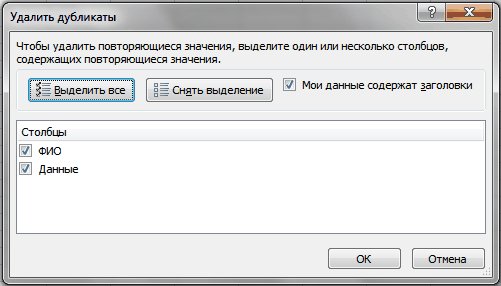
Check the boxes in front of those columns, duplicates in which you want to delete and click OK. If data headers are also located in the selected range, then it is better to set the flag My data contains headers to avoid accidentally deleting data in the table (if they suddenly completely coincide with the value in the title).
Method 1: Advanced filter
In the case of Excel 2003, things are more complicated. There is no such tool as Remove duplicates... But on the other hand, there is such a wonderful tool as Advanced filter... In 2003 this tool can be found in Data -Filter -Advanced filter... The beauty of this method is that you can use it to create a list in a different range rather than spoil the original data. In 2007-2010 Excel, it is also there, but a little hidden. Located on the tab Data, group Sort & Filter - Advanced
How to use it: launch the specified tool - a dialog box appears: 
- Treatment: We choose Copy the result to another location.
- List range: Selecting a range with data (in our case it is A1: A51).
- Criteria range: in this case, leave it blank.
- Copy to range: we indicate the first cell for displaying data - any empty (in the picture - E2).
- Check the box Unique records only.
- We press OK.
Note: if you want to place the result on another sheet, then you simply cannot specify another sheet. You will be able to specify a cell on another sheet, but ... Alas and ah ... Excel will give a message that it cannot copy data to other sheets. But this can also be circumvented, and quite simply. You just need to run Advanced filter from the sheet on which we want to place the result. And as the initial data, we select data from any sheet - this is permissible.
You can also not transfer the result to other cells, but filter the data in place. The data will not be affected in any way - it will be the usual data filtering.
To do this, you just need to select in the Processing section Filter the list, in-place.
Method 2: Formulas
This method is more difficult to understand for inexperienced users, but it creates a list of unique values without changing the original data. Well, it is also more dynamic: if you change the data in the source table, the result will also change. This is sometimes useful. I will try to explain on my fingers what and what: for example, you have a list with data in column A (A1: A51, where A1 is a heading). We will display the list in column C, starting from cell C2. The formula in C2 will be as follows:
(= INDEX ($ A $ 2: $ A $ 51; SMALL (IF (COUNTIF ($ C $ 1: C1; $ A $ 2: $ A $ 51) = 0; ROW ($ A $ 1: $ A $ 50)); 1)) )
(= INDEX ($ A $ 2: $ A $ 51; SMALL (IF (COUNTIF ($ C $ 1: C1; $ A $ 2: $ A $ 51) = 0; ROW ($ A $ 1: $ A $ 50)); 1)) )
A detailed analysis of the operation of this formula is given in the article:
It should be noted that this formula is an array formula. This can be said braces, in which this formula is enclosed. And such a formula is entered into a cell with a keyboard shortcut - Ctrl+Shift+Enter... After we have entered this formula in C2, we must copy and paste it in several lines so as to accurately display all the unique elements. As soon as the formula in the bottom cells returns #NUMBER!- this means all the elements are displayed and there is no point in stretching the formula below. To avoid the error and make the formula more universal (without stretching each time until the error appears), you can use a simple check:
for Excel 2007 and above:
(= IFERROR (INDEX ($ A $ 2: $ A $ 51; SMALL (IF (COUNTIF ($ C $ 1: C1; $ A $ 2: $ A $ 51) = 0; STRING ($ A $ 1: $ A $ 50)); 1 )); ""))
(= IFERROR (INDEX ($ A $ 2: $ A $ 51; SMALL (IF (COUNTIF ($ C $ 1: C1; $ A $ 2: $ A $ 51) = 0; ROW ($ A $ 1: $ A $ 50)); 1 )); ""))
for Excel 2003:
(= IF (ISH (SMALL (IF (COUNTIF ($ C $ 1: C1; $ A $ 2: $ A $ 51) = 0; ROW ($ A $ 1: $ A $ 50)); 1)); ""; INDEX ( $ A $ 2: $ A $ 51; SMALL (IF (COUNTIF ($ C $ 1: C1; $ A $ 2: $ A $ 51) = 0; ROW ($ A $ 1: $ A $ 50)); 1))))
(= IF (ISERR (SMALL (IF (COUNTIF ($ C $ 1: C1; $ A $ 2: $ A $ 51) = 0; ROW ($ A $ 1: $ A $ 50)); 1)); ""; INDEX ( $ A $ 2: $ A $ 51; SMALL (IF (COUNTIF ($ C $ 1: C1; $ A $ 2: $ A $ 51) = 0; ROW ($ A $ 1: $ A $ 50)); 1))))
Then instead of an error #NUMBER! (#NUM!) you will have empty cells(not completely empty, of course - with formulas :-)).
A little more detail about the differences and nuances of the formulas ESLIOSHIBKA and IF (EOSH can be read in this article: How to show 0 in a cell with a formula instead of an error
Method 3: VBA code
This approach will require resolution of macros and basic knowledge of working with them. If you are not sure of your knowledge, I recommend reading these articles first:
- What is a macro and where can I find it? a video tutorial is attached to the article
- What is a module? What modules are there? will be required to figure out where to insert the codes below
Both of the below codes should be placed in standard module... Macros must be allowed.
Let's leave the initial data in the same order - the list with the data is located in column "A" (A1: A51, where A1 is the heading)... Only we will display the list not in column C, but in column E, starting from cell E2:
Sub Extract_Unique () Dim vItem, avArr, li As Long ReDim avArr (1 To Rows.Count, 1 To 1) With New Collection On Error Resume Next For Each vItem In Range ("A2", Cells (Rows.Count, 1) .End (xlUp)). Value "(! LANG: Cells (Rows.Count, 1) .End (xlUp) - defines the last filled cell in column A. Add vItem, CStr (vItem) If Err = 0 Then li = li + 1: avArr (li, 1) = vItem Else: Err.Clear End If Next End With If li Then .Resize (li) .Value = avArr End Sub
With this code, you can extract unique values not only from one column, but from any range of columns and rows. If instead of the line
Range ("A2", Cells(Rows.Count, 1).End(xlUp)).Value !}
specify Selection.Value, then the result of the code will be a list of unique elements from the range selected on the active sheet. Only then would it be nice to change the output cell of values - instead of
put the one in which there is no data.
You can also specify a specific range:
Range ("C2", Cells (Rows.Count, 3). End (xlUp)). Value
Universal code for selecting unique values
The code below can be applied to any ranges. It is enough to run it, specify a range with values for selecting only non-repeating ones (more than one column is allowed) and a cell for displaying the result. The specified cells will be scanned, of which only unique values(empty cells are skipped) and the resulting list will be written starting from the specified cell.
| Sub Extract_Unique () Dim x, avArr, li As Long Dim avVals Dim rVals As Range, rResultCell As Range On Error Resume Next "request the address of the cells to select unique values Set rVals = Application.InputBox ( "Specify a range of cells to sample unique values", "Request Data", "A2: A51", Type: = 8) If rVals Is Nothing Then "if the Cancel button is clicked Exit Sub End If "if only one cell is specified, there is no point in choosing If rVals.Count = 1 Then MsgBox "To filter unique values, you need to specify more than one cell", vbInformation, "www.site" Exit Sub End If "cut off empty rows and columns outside the working range Set rVals = Intersect (rVals, rVals.Parent.UsedRange) "if only empty cells outside the working range are specified If rVals Is Nothing Then MsgBox "Insufficient data to select values", vbInformation, "www.site" Exit Sub End If avVals = rVals.Value "request a cell to display the result Set rResultCell = Application.InputBox ( "Specify a cell to insert the selected unique values", "Request Data", "E2", Type: = 8) If rResultCell Is Nothing Then "if the Cancel button is clicked Exit Sub End If "define the maximum possible dimension of the array for the result ReDim avArr (1 To Rows.Count, 1 To 1) "using a Collection object "select only unique records, "because Collections cannot contain duplicate values With New Collection On Error Resume Next For Each x In avVals If Len (CStr (x)) Then "skip empty cells.Add x, CStr (x) "if the added element already exists in the Collection, an error will occur "if there is no error, this value has not yet been entered, "add to the resulting array If Err = 0 Then li = li + 1 avArr (li, 1) = x Else "be sure to clear the Error object Err.Clear End If End If Next End With "write the result to the sheet, starting from the specified cell If li Then rResultCell.Cells (1, 1) .Resize (li) .Value = avArr End Sub |
Sub Extract_Unique () Dim x, avArr, li As Long Dim avVals Dim rVals As Range, rResultCell As Range On Error Resume Next "request the address of the cells to select unique values Set rVals = Application.InputBox (" Specify the range of cells to select unique values " , "Request for data", "A2: A51", Type: = 8) If rVals Is Nothing Then "if the Cancel button is clicked Exit Sub End If" if only one cell is specified, it makes no sense to select If rVals.Count = 1 Then MsgBox " To select unique values, you need to specify more than one cell ", vbInformation," www.site "Exit Sub End If" cut off empty rows and columns outside the working range Set rVals = Intersect (rVals, rVals.Parent.UsedRange) "if only empty cells are specified out of working range If rVals Is Nothing Then MsgBox "Not enough data to select values", vbInformation, "www..Value" (! LANG: request a cell to display the result Set rResultCell = Application.InputBox ("Укажите ячейку для вставки отобранных уникальных значений", "Запрос данных", "E2", Type:=8) If rResultCell Is Nothing Then "если нажата кнопка Отмена Exit Sub End If "определяем максимально возможную размерность массива для результата ReDim avArr(1 To Rows.Count, 1 To 1) "при помощи объекта Коллекции(Collection) "отбираем только уникальные записи, "т.к. Коллекции не могут содержать повторяющиеся значения With New Collection On Error Resume Next For Each x In avVals If Len(CStr(x)) Then "пропускаем пустые ячейки.Add x, CStr(x) "если добавляемый элемент уже есть в Коллекции - возникнет ошибка "если же ошибки нет - такое значение еще не внесено, "добавляем в результирующий массив If Err = 0 Then li = li + 1 avArr(li, 1) = x Else "обязательно очищаем объект Ошибки Err.Clear End If End If Next End With "записываем результат на лист, начиная с указанной ячейки If li Then rResultCell.Cells(1, 1).Resize(li).Value = avArr End Sub!}
Method 4: pivot tables
Several non-standard way retrieving unique values.
- Select one or more columns in the table, go to the tab Insert-group Table -PivotTable
- In the dialog box Create PivotTable we check the correctness of the selection of the data range (or set new source data)
- indicate the location of the Pivot Table:
- New Worksheet
- Existing Worksheet
- confirm creation by pressing a button OK
Because pivot tables, when processing data that are placed in the area of rows or columns, select only unique values from them for further analysis, then absolutely nothing is required from us except to create a pivot table and place the data of the desired column in the area of rows or columns.
Using the file attached to the article as an example, I:

What is the inconvenience of working with pivot tables in this case: if the source data changes, the pivot table will have to be updated manually: Select any cell of the pivot table - Right mouse button - Refresh or tab Data -Refresh all -Refresh... And if the source data is replenished dynamically and even worse, it will be necessary to re-specify the range of the source data. And one more disadvantage - the data inside the pivot table cannot be changed. Therefore, if it will be necessary to work with the resulting list in the future, then after creating desired list using the summary, it must be copied and pasted on the desired sheet.
To better understand all the steps and learn how to use pivot tables, I strongly recommend that you read the article General information about pivot tables - a video tutorial is attached to it, in which I clearly demonstrate the simplicity and convenience of working with the basic features of pivot tables.
In the attached example, in addition to the described techniques, a slightly more complex variation of extracting unique elements by formula and code is written, namely: extraction of unique elements by criterion... What we are talking about: if in one column of the last name, and in the second (B) there is some data (in the file these are months) and you want to extract the unique values of column B only for the selected last name. Examples of such unique extractions are located on the sheet Extract by criterion.
Download example:
(108.0 KiB, 14,152 downloads)
Did the article help? Share the link with your friends! Video lessons


