Excel data comparison. How to compare two columns in Excel on coincidence

Reading this article will take about 10 minutes. In the next 5 minutes, you can easily compare two columns in Excel and learn about the presence of duplicate in them, remove them or allocate in color. So, time went!

Excel is a very powerful and really cool application for creating and processing large data arrays. If you have several workbooks with data (or only one huge table), then you probably want to compare 2 columns, find repeating values, and then make any actions with them, for example, delete, highlight the color or clear the contents . Columns can be in the same table, be adjacent or not adjacent, can be located on 2 different sheets or even in different books.

Imagine that we have 2 columns with the names of people - 5 names in the column A. and 3 name in column B.. You must compare the names in these two columns and find repeating. As you understand, this is a fictional data taken exclusively for example. In real tables, we are dealing with thousands, and even with tens of thousands of records.

Option A: Both columns are on one sheet. For example, column A. and column B..

Option in: Columns are located on different sheets. For example, column A. On Sheet Sheet2. and column A. On Sheet Sheet3..

In Excel 2013, 2010 and 2007 there is a built-in tool Remove Duplicate. (Delete duplicates), but it is powerless in such a situation, because it cannot compare the data in 2 columns. Moreover, it can only remove duplicates. Other options, such as selection or color change, is not provided. And the point!

Compare 2 columns in Excel and find repetitive entries with formulas

Option A: Both columns are on one sheet

Prompt: In large tables, copy the formula will be faster if you use key combinations. Highlight the cell C1. and press Ctrl + C. (To copy the formula to the clipboard), then click Ctrl + Shift + End (To allocate all non-empty cells in the column C) and, finally, click Ctrl + V. (To insert a formula into all selected cells).

Option Q: Two columns are on different sheets (in different books)

Processing of the found duplicates

Excellent, we found entries in the first column, which are also present in the second column. Now we need to do something with them. View all repetitive entries in the table manually quite inefficient and takes too much time. There are ways better.

Show only repetitive lines in column A

If your columns do not have headers, then you need to add. To do this, place the cursor on the number indicating the first line, while it will turn into a black arrow, as shown in the figure below:

Right-click and select the context menu. Insert. (Paste):

Give titles to columns, for example, " Name."And" Duplicate?"Then open the tab Data. (Data) and click Filter. (Filter):

After that, press the little gray arrow next to " Duplicate?"To uncover the filter menu; remove the checkboxes from all the items of this list, except Duplicate., and press OK.

That's all, now you see only those elements of the column BUTwho are duplicated in column IN. In our tutorial table there are only two such cells, but as you understand, in practice they will meet much more.

To display all the column lines again BUT, click the filter symbol in the column INwhich now looks like a funnel with a small arrow and select Select all. (Select all). Or you can do the same through the tape by clicking Data. (Data)\u003e Select & Filter. (Sorting and filter)\u003e Clear (Clear), as shown in the screen shot below:

Changing the color or selection of found duplicates

If noting " Duplicate."Not enough for your goals, and you want to mention repeating cells to other color font, fill or in any other way ...

In this case, filter the duplicates, as shown above, highlight all filtered cells and click Ctrl + 1.to open the dialog box Format Cells. (Cell format). As an example, let's change the color of the cells of the cells in rows with duplicates on bright yellow. Of course, you can change the color of the fill with the tool FILL (Fill color) on the tab HOME (Home), but the advantage of the dialog box Format Cells. (Cell format) is that all formatting parameters can be configured simultaneously.

Now you definitely do not miss any cell with duplicates:

Removing repetitive values \u200b\u200bfrom the first column

Filter the table so that only cells with repeating values \u200b\u200bwere shown, and highlight these cells.

If the 2 columns that you compare are on different sheets, that is, in different tables, right-click the dedicated range and in the context menu, select Delete Row (Delete a string):

Click OKWhen Excel asks you to confirm that you really want to delete the entire line of the sheet and then clean the filter. As you can see, there are only rows with unique values:

If 2 columns are located on one sheet, close to each other (adjacent) or not close to each other (not adjacent), the process of removing duplicates will be slightly complicated. We cannot remove the entire row with repeating values, because we remove the cells and from the second column too. So to leave only unique entries in the column BUTMake the following:

As you can see, remove duplicates from two columns in Excel with the help of formulas is not so difficult.

Quite often, Excel users have a task of comparing two tables or lists to identify differences in them or missing items. Each user copes with this task in its own way, but most often a rather large amount of time is spent on solving the specified question, since not all approaches to this problem are rational. At the same time, there are several proven actions algorithms that will allow compare lists or table arrays in fairly short time with minimal considerable effort. Let's consider details these options.

There are quite a few ways to compare table areas in Excel, but all of them can be divided into three large groups:

comparison of lists on one sheet;

comparison of tables located on different sheets;

comparison of tables in different files.

It is based on this classification, first of all, the comparison methods are selected, and specific actions and algorithms are determined to perform the task. For example, when comparing, in different books, two Excel files are required simultaneously.

In addition, it should be said that to compare the tabular areas makes sense only when they have a similar structure.

Method 1: Simple Formula

The easiest way to compare data in two tables is the use of a simple formula of equality. If the data coincides, then it gives the indicator of truth, and if not, then - a lie. You can compare, both numeric data and text. The disadvantage of this method is that it can only be used if the data in the table is ordered or sorted equally, synchronized and have an equal number of lines. Let's see how to use this method in practice on the example of two tables placed on one sheet.

So, we have two simple tables with lists of enterprise employees and their salary. You need to compare the list of employees and identify inconsistencies between columns in which the names are located.

To do this, we will need an additional column on the sheet. Enter the sign there «=» . Then click on the first name, which must be compared in the first list. Again set the symbol «=» from the keyboard. Next, click on the first cell of the column, which we compare in the second table. It turned out the expression of the following type:

Although, of course, in each case, the coordinates will differ, but the essence will remain the same.
Click on the key ENTERto get the results of the comparison. As you can see, when comparing the first cells of both lists, the program indicated the indicator "TRUE"What does the data coincide.

Now we need to carry out a similar operation and with the other cells of both tables in the columns that we compare. But you can simply copy the formula, which will allow to significantly save time. This factor is especially important when comparing lists with a large number of lines.
The copying procedure is easiest to complete with a filling marker. We bring the cursor to the right lower corner of the cell, where we received an indicator "TRUE". At the same time, he must transform into a black cross. This is a filling marker. We click the left mouse button and pull the cursor down on the number of lines in the tables compared to the table arrays.

As you can see, now the additional column displays all the results of the data comparison in two columns of table arrays. In our case, the data did not coincide only in one row. With their comparison, the formula issued the result "FALSE". For all other stricters, as you can see, the comparison formula issued an indicator "TRUE".

In addition, there is an opportunity with the help of a special formula to calculate the number of discrepancy. To do this, we highlight the element of the sheet where it will be output. Then click on the icon "Insert a function".

In the window Masters functions in the group of operators "Mathematical" Allocate the name Summipa. Click on the button Ok.

The function arguments window is activated. SummipaThe main task of which is to calculate the amount of the dedicated range. But this feature can be used for our purposes. She is quite simple syntax:
Summaging (array1; array2; ...)

In total, addresses up to 255 arresses can be used as arguments. But in our case, we will use only two arrays, besides, as one argument.

Put the cursor in the field "Massive1" and allocate a compared data range in the first area on the sheet. After that, in the field put a sign "not equal" (<> ) and allocate a compared range of the second area. Next, we sell the resulting expression with brackets, in front of which we put two characters «-» . In our case, it turned out such an expression:

- (A2: A7<>D2: D7)

Click on the button Ok.

The operator makes the calculation and displays the result. As we see, in our case, the result is equal to the number "one"That is, it means that one incompariety was found in compared lists. If the lists were completely identical, then the result would be equal to the number «0» .

In the same way, you can compare the data in the tables that are located on different sheets. But in this case, it is desirable that the lines in them are numbered. The rest of the comparison procedure is almost exactly the same as described above, besides the fact that when making the formula, it is necessary to switch between sheets. In our case, the expression will have the following form:

B2 \u003d List2! B2

That is, as we see, in front of the data coordinates, which are located on other sheets other than where the comparison result is displayed, the sheet number and an exclamation mark is indicated.

Method 2: Selection of groups of cells

Comparison can be made using the tool for the separation of groups of cells. With it, you can also compare only synchronized and ordered lists. In addition, in this case, lists must be located next to each other on one sheet.

Method 3: Conditional Formatting

You can make a comparison by applying conditional formatting method. As in the previous method, compared areas should be on a single Excel working sheet and be synchronized with each other.

There is another way to apply conditional formatting to perform the task. Like the previous options, it requires the location of both compared areas on one sheet, but in contrast to the previously described methods, the synchronization condition or sorting data will not be compulsory, which distinguishes this option from previously described.

If you wish, you can, on the contrary, paint the inconsistent elements, and the indicators that match, leave with the fill of the previous color. At the same time, the algorithm of action is almost the same, but in the settings window allocate the repetitive values \u200b\u200bin the first field instead of the parameter "Repeating" You should select a parameter "Unique". After that click on the button Ok.

Thus, it is precisely those indicators that do not coincide.

Method 4: Comprehensive Formula

Also compare the data with the help of a complex formula, the basis of which is the function Countess. Using this tool, you can calculate how much each element from the selected column of the second table is repeated in the first.

Operator Countess refers to the statistical group of functions. Its task is to count the number of cells, the values \u200b\u200bin which satisfy the specified condition. The syntax of this operator has this kind:

Schedule (Range; Criterion)

Argument "Range" It represents the address of the array, which calculates the coincident values.

Argument "Criterion"sets the condition of the coincidence. In our case, it will be the coordinates of the specific cells of the first tabular area.

Of course, this expression in order to compare table indicators, it is possible to apply in the existing form, but it is possible to improve it.

We will make that the values \u200b\u200bthat exist in the second table, but are not available in the first, were displayed as a separate list.

First of all, we recycle our formula Countess, namely we will make it one of the operator arguments IF A. To do this, select the first cell in which the operator is located Countess. In the line formulas in front of it add expression "IF A" Without quotes and open brackets. Next, so that it is easier for us to work, allocate the value in the line formula "IF A" and click on the icon "Insert a function".

Opened function arguments IF A. As you can see, the first window of the window has already been filled with the operator's value. Countess. But we need to add something else in this field. We install the cursor and the already existing expression add «=0» without quotes.
After that go to the field "Meaning if truth". Here we will use another nested function - LINE. Enter the Word "LINE" Without quotes, further open brackets and indicate the coordinates of the first cell with the surname in the second table, after which we close brackets. Specifically in our case in the field "Meaning if truth" It turned out the following expression:

Row (D2)

Now operator LINE will report functions IF A The number of the string in which the specific surname is located, and in the case when the condition specified in the first field will be performed, the function IF A Will output this number in the cell. Click on the button Ok.

As you can see, the first result is displayed as "FALSE". This means that the value does not satisfy the conditions of the operator IF A. That is, the first surname is present in both lists.

Using the filling marker, the already familiar way copying the expression of the operator IF A On the whole column. As we see, in two positions that are present in the second table, but not in the first, the formula issues rows numbers.

Retreat from the table area to the right and fill in the column numbers in order, ranging from 1 . The number of rooms must coincide with the number of rows in the second compaable table. To speed up the numbering procedure, you can also use the fill marker.

After that, we highlight the first cell to the right of the speaker with the numbers and click on the icon "Insert a function".

Opens Master of Functions. Go to category "Statistical" and make a choice of name "LEAST". Click on the button Ok.

Function LEASTThe window of the arguments of which was disclosed, intended to withdraw the specified smallest value.
In field "Array" You should specify the coordinates of the range of the additional column "Number of coincidences"which we previously transformed using the function IF A. We make all links absolute.

In field "K" It is indicated what the least value should be displayed. Here we indicate the coordinates of the first cell of the column with the numbering, which we recently added. Address Leave relative. Click on the button Ok.

The operator displays the result - the number 3 . It is it that is the smallest of the numbering of the inconsistent lines of table arrays. Using the filling marker, copy the formula to the nose itself.

Now, knowing the rows of the incomprehensive elements, we can insert into the cell and their values \u200b\u200busing the function INDEX. Select the first element of the sheet containing the formula LEAST. After that, go to the formula string and before the name "LEAST" Add name "INDEX" Without quotes, immediately open the bracket and put a point with a comma ( ; ). Then we highlight the formula name in the line "INDEX" and click on pictogram "Insert a function".

After that, a small window opens, in which it is necessary to determine if the reference should have a function INDEX or designed to work with arrays. We need a second option. It is installed by default, so that in this window just click on the button Ok.

The function arguments window starts INDEX. This operator is designed to output a value that is located in a specific array in the specified line.
As you can see the field "Row number" Already filled with function values LEAST. From an existing value there, the difference between the numbering of the Excel sheet and the internal numbering of the tabular region. As we see, we only have a hat on the table values. This means that the difference is one line. So add in the field "Row number" value "-one" without quotes.

In field "Array" Indicate the address of the range of values \u200b\u200bof the second table. At the same time, all the coordinates make absolute, that is, we put the dollar sign before the method described by us.

Click on the button Ok.

After withdrawing, the result on the screen is stretching the function using the fill marker to the end of the column down. As we see, both surnames that are present in the second table, but are not available in the first, are removed in a separate range.

Method 5: Comparison of arrays in different books

When comparing the ranges in different books, you can use the above methods, excluding those options where the placement of both tabular areas on one sheet is required. The main condition for the comparison procedure in this case is the opening of the windows of both files at the same time. For versions of Excel 2013 and later, as well as for versions to Excel 2007, there are no problems with the implementation of this condition. But in Excel 2007 and Excel 2010 in order to open both windows at the same time, additional manipulations are required. How to do it tells in a separate lesson.

As you can see, there are a number of possibilities to compare tables with each other. What kind of option to use depends on where the table data relative to each other is located (on one sheet, in different books, on different sheets), as well as from the user wants this comparison to be displayed on the screen.

Say You Want to Compare Versions of a Workbook, Analyze A Workbook for Problems or Inconsistencies, Or See Links Between Workbooks or Worksheets. If Microsoft Office 365 Or Office Professional Plus 2013 IS Installed On Your Computer, The Spreadsheet Inquire Add-in Is Available in Excel.

You can Use the Commands in the inquire tab to do all these Tasks and More. The Inquire Tab On The Excel Ribbon Has Buttons For the Commands Described Below.

If you don "t See the Inquire. Tab In The Excel Ribbon, See Turn on the Spreadsheet Inquire Add-in.

Compare Two Workbooks.

Their Compare Files. Command Lets You See The Differences, Cell by Cell, Between Two Workbooks. You Need to Have Two Workbooks Open In Excel to Run This Command.

Results Are Color Coded by The Kind Of Content, Such As Entered Values, Formulas, Named Ranges, And Formats. There "s Even A Window That Can Show VBA Code Changes Line by Line. Differences Between Cells Are Shown in An Easy to Read Grid Layout, Like this:

Their Compare Files. Command Use Microsoft Spreadsheet Compare to Compare The Two Files. In Windows 8, You Can Start Spreadsheet Compare Outside Of Excel By Clicking Spreadsheet Compare. ON THE Apps. Screen. In Windows 7, Click The Windows Start. Button and then\u003e All Programs > Microsoft Office 2013. > Office 2013 Tools. > Spreadsheet Compare 2013..

To Learn More About Spreadsheet Compare and Comparing Files, Read Compare Two Versions of a Workbook.

Analyze a workbook.

Their Workbook Analysis. Command Creates An Interactive Report Showing Detailed Information About the Workbook and Its Structure, Formulas, Cells, Ranges, And Warnings. The Picture Here Shows a Very Simple Workbook Containing Two Formulas and Data Connections to An Access Database and a Text File.

Show Workbook Links.

Cell Cell Cell Cell Cell Cell Cell Cell Cell Cell Cell Cell Cell Cell Connected to Oterbookes. Use The to Create An Interactive, Graphical Map of Workbook Dependencies Created by Connections (Links) Between Files. The Types of Links In The Diagram Can Include Other Workbooks, Access Databases, Text Files, Html Pages, SQL Server Databases, and Other Data Sources. In The Relationship Diagram, You Can Select Elements and Find More Information ABout Them, and Drag Connection Lines to Change the Shape Of the Diagram.

This Diagram Shows The Current Workbook on The Left And The Connections Between It and Other Workbooks and Data Sources. IT ALSO SHOWS ADDITIONAL LEVELS OF WORKBOOK CONNECTIONS, GIVING YOU A PICTURE OF THE DATA ORIGINS FOR THE WORKBOOK.

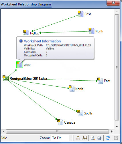
Show Worksheet Links.

Got Lots of Worksheets That Depend ON Each Other? Use The to Create An Interactive, Graphical Map of Connections (Links) Between Worksheets Both In The Same Workbook and in Oter Workbooks. This Helps Give You A Clearer Picture of How Your Data Might Depend On Cells in Other Places.

This Diagram Schows The Relationships Between Worksheets in Four Different Workbooks, with Dependencies Between Worksheets In The Same Workbook As Well As Links Between Worksheets in Different Workbooks. WHEN YOU POSITION Your Pointer Over A Node In The Diagram, Such As The Worksheet Named "West" In The Diagram, a Balloon Containing Information Appears.

Show Cell Relationships.

To Get A Detailed, Interactive Diagram of All Links From a Selected Cell to Cells in Other Worksheets or Even Other WorkBooks, USE Cell Relationship. Tool. These Relationships with Other Cells Can Exist in Formulas, or References to Named Ranges. The Diagram Can Cross Worksheets and Workbooks.

This Diagram Shows Two Levels of Cell Relationships for Cell A10 on Sheet5 in Book1.xlsx. This Cell Is Dependent On Cell C6 On Sheet 1 In Another Workbook, Book2.xlsx. This Cell Is A Precedent for Several Cells on Other Worksheets in The Same File.

To Learn More about Viewing Cell Relationships, Read See Links Between Cells.

Clean Excess Cell Formatting

Ever Open A Workbook and Find IT Loads Slowly, Or Have Become Huge? IT Might Have Formatting AppLied to Rows or Columns You Aren "T Aware Of. Use the Clean Excess Cell Formatting Command to Remove Excess Formatting and Greatly Reduce File Size. This Helps You Avoid "Spreadsheet Bloat," Which Imprives Excel "S Speed.

MANAGE PASSWORDS.

If You "Re USING THE INQUIRE FEATURES TO ANALYZE OR COMPARE WORKBOOKS TAAT ARE PASSWORD PROTECTED, YOU" LL Need to Add The Workbook Password to Your Password List So That Inquire Can Open The Saved Copy of Your Workbook. Use the Workbook Passwords. Command on the Inquire. Tab to Add Passwords, Which Will Be Saved on Your Computer. These Passwords Are Encrypted and Only Accessible by You.

The article gives any answers to the following questions:

How to compare two tables in Excel?
How to compare complex tables in Excel?
How to make a comparison of tables in Excel using the VD () function?
How to form unique lines identifiers if their uniqueness is initially determined by the set of values \u200b\u200bin several columns?
How to fix the values \u200b\u200bof cells in formulas when copying formulas?

When working with large amounts of information, the user may encounter such a task as a comparison of two tabular data sources. When storing data in a single accounting system (for example, a system based on 1C enterprise, systems using SQL databases), built-in or DBMS can be used to compare the data. As a rule, this is enough to attract a programmer that will write a request to the database, or the reporting mechanism of the report. An experienced user who owns the skill of writing requests 1c or SQL can cope with the query.

Problems begin when it is necessary to perform the task of the comparison of the data urgently, and the programmer attracting and writing them the query or program report may exceed the time limit set for solving the task. Another equally widespread problem is the need to compare information from various sources. In this case, the setting of the task for the programmer will sound as the integration of two systems. The solution to such a task will require a higher qualification of the programmer and will also take longer than the development in a single system.

To solve the designated problems, the perfect reception is to use to compare the data of the Microsoft Excel tabular editor. Most common management and regulated accounting systems maintain unloading to Excel format. This task will require only a certain user qualification for working with this office package and will not require programming skills.

Consider the solution of the task of comparing tables in Excel on the example. We have two tables containing lists of apartments. Sources of unloading - 1C Enterprise (construction accounting) and a table in Excel (sales accounting). Tables are located in the Excel workbook on the first and second sheets, respectively.

We have a task to compare these lists at. In the first table - all apartments at home. In the second table - only sold apartments and the name of the buyer. The ultimate goal is to display in the first table for each apartment the name of the buyer (for those apartments that were sold). The task is complicated by the fact that the address of the apartment in each table is construction and consists of several fields: 1) Case address (at home), 2) Section (entrance), 3) Floor, 4) Room on the floor (for example, from 1 to 4) .

To compare the two Excel tables, we need to achieve that in both tables each line it would be identified with one field, and not four. You can get such a field by connecting the values \u200b\u200bof four address fields by the Capture Function (). Purpose Function Catch () - Combining multiple text values \u200b\u200bto one line. Values \u200b\u200bin the functions are listed through the ";" symbol. As values, both cell addresses and arbitrary text specified in quotes can appear as values.

Step 1. Insert the empty column "A" at the beginning of the first table and in the cell of this column opposite the first line with the data formula:
\u003d Catch (B3; "-"; C3; "-"; D3; "-"; E3)
For the convenience of visual perception between the values \u200b\u200bof the cells of the cells, we set the characters "-".

Step 2. Copy the formula in the following cells of the column A.

Step 4. To compare Excel tables by values, use the PRD () function. Assigning the PRD () function - search for values \u200b\u200bin the extreme left column of the table and return the value of the cell located in the specified column of the same string. The first parameter is the desired value. The second parameter is a table in which the search will be found. The third parameter is the column number, from the cell of which the value will be returned in the found line. The fourth parameter is the type of search: a lie - the exact coincidence, the truth is an approximate coincidence. Since the output should be placed in the first table (it was necessary to add buyers' names), then we will prescribe the formula in it. We form in the free column to the right of the table opposite the first line of these formula:
\u003d VD (A3; List2! $ A $ 3: $ F $ 10; 6; lie)
When copying the Smart formula, Excel automatically changes the addressing cells. In our case, the desired value for each row will be changed: A3, A4, etc., and the address of the table in which the search is conducted should remain unchanged. To do this, fix the cells in the address parameter of the table "$" symbols. Instead of "sheet2! A3: F10" Make "list2! $ A $ 3: $ F $ 10".

After installing the superstructure, you will have a new tab with the function call command. Pressing the command Comparison of ranges A dialog box appears for entering parameters.

This macro allows you to compare tables of any volume and with any number of columns. Comparison of tables can be carried out by one, two or three columns at the same time.

The dialog box is divided into two parts: the left for the first table and the right for the second.

To compare tables, you must perform the following steps:

Specify tables of tables.
Set the checkbox (check / bird) under the selected range of the tables if the table includes a header (header string).
Select columns of the left and right table for which the comparison will be carried out (if the ranges of the tables do not include the columns headers will be numbered).
Specify the type of comparison.
Select option for issuing results.

Type of comparing tables

The program allows you to select multiple types of table comparisons:

Find lines of one table that are missing in another table

When this type of comparison is selected, the program is looking for lines of one table that are missing in another. If you are mapping a table in several columns, then the result will be the lines in which there is a distinction for at least one of the columns.

Find matching strings

When this type of comparison is selected, the program finds the strings that match the first and second tables. The strokes in which the values \u200b\u200bin the selected comparison columns (1, 2, 3) are completely coincided with the values \u200b\u200bof the second table columns.

An example of the program in this mode is presented to the right in the picture.

Match table based on selected

In this comparison mode, opposite each row of the first table (selected as the main), the data of the matching line of the second table is copied. In the event that there are no matching lines, the line opposite the main table remains empty.