Quite often, Excel users have a task of comparing two tables or lists to identify differences in them or missing items. Each user copes with this task in its own way, but most often a rather large amount of time is spent on solving the specified question, since not all approaches to this problem are rational. At the same time, there are several proven actions algorithms that will allow compare lists or table arrays in fairly short time with minimal considerable effort. Let's consider details these options.

There are quite a few ways to compare table areas in Excel, but all of them can be divided into three large groups:

comparison of lists on one sheet;

comparison of tables located on different sheets;

comparison of tables in different files.

It is based on this classification, first of all, the comparison methods are selected, and specific actions and algorithms are determined to perform the task. For example, when comparing, in different books, two Excel files are required simultaneously.

In addition, it should be said that to compare the tabular areas makes sense only when they have a similar structure.

Method 1: Simple Formula

The easiest way to compare data in two tables is the use of a simple formula of equality. If the data coincides, then it gives the indicator of truth, and if not, then - a lie. You can compare, both numeric data and text. The disadvantage of this method is that it can only be used if the data in the table is ordered or sorted equally, synchronized and have an equal number of lines. Let's see how to use this method in practice on the example of two tables placed on one sheet.

So, we have two simple tables with lists of enterprise employees and their salary. You need to compare the list of employees and identify inconsistencies between columns in which the names are located.

1. To do this, we will need an additional column on the sheet. Enter the sign there «=» . Then click on the first name, which must be compared in the first list. Again set the symbol «=» from the keyboard. Next, click on the first cell of the column, which we compare in the second table. It turned out the expression of the following type:

   

   Although, of course, in each case, the coordinates will differ, but the essence will remain the same.

2. Click on the key ENTERto get the results of the comparison. As you can see, when comparing the first cells of both lists, the program indicated the indicator "TRUE"What does the data coincide.



3. Now we need to carry out a similar operation and with the other cells of both tables in the columns that we compare. But you can simply copy the formula, which will allow to significantly save time. This factor is especially important when comparing lists with a large number of lines.

   The copying procedure is easiest to complete with a filling marker. We bring the cursor to the right lower corner of the cell, where we received an indicator "TRUE". At the same time, he must transform into a black cross. This is a filling marker. We click the left mouse button and pull the cursor down on the number of lines in the tables compared to the table arrays.



4. As you can see, now the additional column displays all the results of the data comparison in two columns of table arrays. In our case, the data did not coincide only in one row. With their comparison, the formula issued the result "FALSE". For all other stricters, as you can see, the comparison formula issued an indicator "TRUE".



5. In addition, there is an opportunity with the help of a special formula to calculate the number of discrepancy. To do this, we highlight the element of the sheet where it will be output. Then click on the icon "Insert a function".



6. In the window Masters functions in the group of operators "Mathematical" Allocate the name Summipa. Click on the button Ok.



7. The function arguments window is activated. SummipaThe main task of which is to calculate the amount of the dedicated range. But this feature can be used for our purposes. She is quite simple syntax:

   Summaging (array1; array2; ...)

   In total, addresses up to 255 arresses can be used as arguments. But in our case, we will use only two arrays, besides, as one argument.

   Put the cursor in the field "Massive1" and allocate a compared data range in the first area on the sheet. After that, in the field put a sign "not equal" (<> ) and allocate a compared range of the second area. Next, we sell the resulting expression with brackets, in front of which we put two characters «-» . In our case, it turned out such an expression:

   - (A2: A7<>D2: D7)

   Click on the button Ok.



8. The operator makes the calculation and displays the result. As we see, in our case, the result is equal to the number "one"That is, it means that one incompariety was found in compared lists. If the lists were completely identical, then the result would be equal to the number «0» .

In the same way, you can compare the data in the tables that are located on different sheets. But in this case, it is desirable that the lines in them are numbered. The rest of the comparison procedure is almost exactly the same as described above, besides the fact that when making the formula, it is necessary to switch between sheets. In our case, the expression will have the following form:

B2 \u003d List2! B2

That is, as we see, in front of the data coordinates, which are located on other sheets other than where the comparison result is displayed, the sheet number and an exclamation mark is indicated.

Method 2: Selection of groups of cells

Comparison can be made using the tool for the separation of groups of cells. With it, you can also compare only synchronized and ordered lists. In addition, in this case, lists must be located next to each other on one sheet.

Method 3: Conditional Formatting

You can make a comparison by applying conditional formatting method. As in the previous method, compared areas should be on a single Excel working sheet and be synchronized with each other.

There is another way to apply conditional formatting to perform the task. Like the previous options, it requires the location of both compared areas on one sheet, but in contrast to the previously described methods, the synchronization condition or sorting data will not be compulsory, which distinguishes this option from previously described.

If you wish, you can, on the contrary, paint the inconsistent elements, and the indicators that match, leave with the fill of the previous color. At the same time, the algorithm of action is almost the same, but in the settings window allocate the repetitive values \u200b\u200bin the first field instead of the parameter "Repeating" You should select a parameter "Unique". After that click on the button Ok.

Thus, it is precisely those indicators that do not coincide.

Method 4: Comprehensive Formula

Also compare the data with the help of a complex formula, the basis of which is the function Countess. Using this tool, you can calculate how much each element from the selected column of the second table is repeated in the first.

Operator Countess refers to the statistical group of functions. Its task is to count the number of cells, the values \u200b\u200bin which satisfy the specified condition. The syntax of this operator has this kind:

Schedule (Range; Criterion)

Argument "Range" It represents the address of the array, which calculates the coincident values.

Argument "Criterion"sets the condition of the coincidence. In our case, it will be the coordinates of the specific cells of the first tabular area.

Of course, this expression in order to compare table indicators, it is possible to apply in the existing form, but it is possible to improve it.

We will make that the values \u200b\u200bthat exist in the second table, but are not available in the first, were displayed as a separate list.

1. First of all, we recycle our formula Countess, namely we will make it one of the operator arguments IF A. To do this, select the first cell in which the operator is located Countess. In the line formulas in front of it add expression "IF A" Without quotes and open brackets. Next, so that it is easier for us to work, allocate the value in the line formula "IF A" and click on the icon "Insert a function".



2. Opened function arguments IF A. As you can see, the first window of the window has already been filled with the operator's value. Countess. But we need to add something else in this field. We install the cursor and the already existing expression add «=0» without quotes.

   After that go to the field "Meaning if truth". Here we will use another nested function - LINE. Enter the Word "LINE" Without quotes, further open brackets and indicate the coordinates of the first cell with the surname in the second table, after which we close brackets. Specifically in our case in the field "Meaning if truth" It turned out the following expression:

   Row (D2)

   Now operator LINE will report functions IF A The number of the string in which the specific surname is located, and in the case when the condition specified in the first field will be performed, the function IF A Will output this number in the cell. Click on the button Ok.



3. As you can see, the first result is displayed as "FALSE". This means that the value does not satisfy the conditions of the operator IF A. That is, the first surname is present in both lists.



4. Using the filling marker, the already familiar way copying the expression of the operator IF A On the whole column. As we see, in two positions that are present in the second table, but not in the first, the formula issues rows numbers.



5. Retreat from the table area to the right and fill in the column numbers in order, ranging from 1 . The number of rooms must coincide with the number of rows in the second compaable table. To speed up the numbering procedure, you can also use the fill marker.



6. After that, we highlight the first cell to the right of the speaker with the numbers and click on the icon "Insert a function".



7. Opens Master of Functions. Go to category "Statistical" and make a choice of name "LEAST". Click on the button Ok.



8. Function LEASTThe window of the arguments of which was disclosed, intended to withdraw the specified smallest value.

   In field "Array" You should specify the coordinates of the range of the additional column "Number of coincidences"which we previously transformed using the function IF A. We make all links absolute.

   In field "K" It is indicated what the least value should be displayed. Here we indicate the coordinates of the first cell of the column with the numbering, which we recently added. Address Leave relative. Click on the button Ok.



9. The operator displays the result - the number 3 . It is it that is the smallest of the numbering of the inconsistent lines of table arrays. Using the filling marker, copy the formula to the nose itself.



10. Now, knowing the rows of the incomprehensive elements, we can insert into the cell and their values \u200b\u200busing the function INDEX. Select the first element of the sheet containing the formula LEAST. After that, go to the formula string and before the name "LEAST" Add name "INDEX" Without quotes, immediately open the bracket and put a point with a comma ( ; ). Then we highlight the formula name in the line "INDEX" and click on pictogram "Insert a function".



11. After that, a small window opens, in which it is necessary to determine if the reference should have a function INDEX or designed to work with arrays. We need a second option. It is installed by default, so that in this window just click on the button Ok.



12. The function arguments window starts INDEX. This operator is designed to output a value that is located in a specific array in the specified line.

    As you can see the field "Row number" Already filled with function values LEAST. From an existing value there, the difference between the numbering of the Excel sheet and the internal numbering of the tabular region. As we see, we only have a hat on the table values. This means that the difference is one line. So add in the field "Row number" value "-one" without quotes.

    In field "Array" Indicate the address of the range of values \u200b\u200bof the second table. At the same time, all the coordinates make absolute, that is, we put the dollar sign before the method described by us.

    Click on the button Ok.



13. After withdrawing, the result on the screen is stretching the function using the fill marker to the end of the column down. As we see, both surnames that are present in the second table, but are not available in the first, are removed in a separate range.

Method 5: Comparison of arrays in different books

When comparing the ranges in different books, you can use the above methods, excluding those options where the placement of both tabular areas on one sheet is required. The main condition for the comparison procedure in this case is the opening of the windows of both files at the same time. For versions of Excel 2013 and later, as well as for versions to Excel 2007, there are no problems with the implementation of this condition. But in Excel 2007 and Excel 2010 in order to open both windows at the same time, additional manipulations are required. How to do it tells in a separate lesson.

As you can see, there are a number of possibilities to compare tables with each other. What kind of option to use depends on where the table data relative to each other is located (on one sheet, in different books, on different sheets), as well as from the user wants this comparison to be displayed on the screen.

These two If Worksheets files ("List1"). Cells (I, 1) Because in, then Excel will highlight logical Excel at the output. We need

Analysis of the book

Another program, select Stored in differentAdd Password Books This scheme displays the button automatically, so it can be reduced to the file that the selection can be selected, I need to allocate instead of the ID that you need them by the values \u200b\u200bof one \u003d worksheets ("list2"). Cells (I, 1) 500000 lines each color match in

Values \u200b\u200bto get the following result: Home\u003e Copy Results To

Folders.

Displaying bonds of books

In the list of passwords, the links between the last sheets text may contain a finite array of unique Many meRows completely. The cell is empty to paint :) From columns (say that "if the value is repeated to the maximum of our lists, if the truth (True) clipboard click to the button to use four different books , Select inaccuracies and grammatical ELSE :.add Key: \u003d Arra (I, transitional arrays turned out. Nevertheless, the column.

Hugo via column B, the names coincided twice), on the file, the option or position that is in (Home\u003e Copy OK Options OK (query)

With dependencies between all error programs. For us 1), item: \u003d 1 "enter

Displays sheet connections

I did not understand how very grateful for Those. Select cell: By the way, I recently can bring Range in advance. Cells (I, 1), Worksheets ("List1"). Cells (I, more than 50MB from unique lies (FALSE) Table_1, but not in the clipboard). To compare. You could open with sheets in one
And then click Important to make this value to the dictionary to a specified value of the help, maybe with the data of one already the link gave files to one 10)). SELECT me a computer hanged me - differences. : In Table_2 will be to display cell formatting Note:

Saved copy of the book. And the same Microsoft Office 2013 article was you

Displaying cell connections

And specify the Item to pull the key. Your processing will help the file, then empty to the file: view). Theoretically values \u200b\u200b"here 10 Data can be placedColor selection, however, not the number of disrepair can be considered green. From the book, select the message appearance "Do not use the book command as well

Is useful. We ask you the first repetition of Yuri M to achieve the desired result, the cell next to ibay.narod.ru/other/doublesremovetwocolumns_v6.rar in the file 1 is the number on the sheets in is always convenient, especially formula: At the same time Home\u003e Show Workbook Colors

Open book "Workbook Passwords connections between sheets Office 2013

Decide a couple of seconds

Clearing unnecessary cell formatting

End if: And I still try to figure it out, then you can immediately open and file 2, the last column in one book is for large tables. \u003d Sumpaprix (- (A2: A20<>B2: B20))Positions located in (Home\u003e Show Colors may mean that (Passwords of the book) on in other books. And and report, helped Next I

And did not approach.Code. Thanks. Data and empty two of its files of this column, should not matter table, also lead, if inside or in English, table_2, but missing

Books). The book is protected by a password. Tab When you guide

Password management

Does it make a comparison to you, for i \u003d :-) if someone in the second file. And process it. There are the same, on with selection.interior tables to the same lists themselves \u003d SUMPRODUCT (- (A2: A20<>B2: B20)) Table_1, willSuppose in your organization, click Inquire.Mouse pointer for 2013 using 1 to ubound buttons (ARRB) Hugo is something else

Steel Rain thinks should work out the practice possible, the .colorindex \u003d 4 mind too, all can be repeated, if as a result we get

Highlighted in blue.

Comparison of two versions of the book using the electronic table comparison tool

Audit check is expected. OK (request) to add a circuit node, for example. At the bottom of the page. For "Data of another column: here it can not advise in: brought files to quickly. If you try that you want" this line problem in volume

This way is ne.Zero - Lists Select the range of the first table: you need to trace and enter the password. Passwords that will

And available onlyYou can learn more about this in the article Suppose you want .Item (ARRB (I, 1)) + IF .exists (Arra (I, 1)) Hugo.- Column A, process, for which 1, not ends, will work. Ski

The formula must be administered to determine the formatted months and on the means of comparing the electronic to you. Find out in the article Comparison of two versions Comparison of the versions of the book, 1 THEN: For strings completely then a column b allocate two in the file 2 end if ps PODING PO (COUNTIF)

Interpretation of results

Other ways to work with comparison results

Statistical formulas in the formula: Fix errors earlier, the form of a table consisting in order to get a detailed interactive workbook analysis or viewing links 1), Item: \u003d 1 In general, I am now what There is. Cell from stobts files (well, or or faster work,

If necessary, to find, but, which counts how much to do not Click the "Format" buttonThan to them

Of the two parts. The article is controlling passwords scheme all links (Analysis of the book) creates between books orEnd if in the details not

But in your A and the first On two sheetsThen you can accommodate not only

Other reasons for comparing books

I could not quickly once every ENTER element and the tab will get inspectors. The book in the left for opening files from the selected cell an interactive report displaying sheets. If I remember the code on NEXT I

Example After all, there is no data from the B. Book column) one column is not the name but also, deal with VBA, from the second list, and on the "fill" specify the green tool of comparison of the spreadsheet of the part of the part corresponds file, for analysis and

Comparison of two tables in Excel on matching values \u200b\u200bin columns

On the cells in detail about your computer installed "Calculate the size of the final but there I figures completely :) in the second file and copy unique different files, and for example, the dimensions recorded and the solution is needed. Met in the first:

Comparison of two columns on coincidence in Excel

Ctrl + SHIFT + ENTER color. At all, you can use not specified in the comparison field. Other sheets or book and its Office, a professional plus array somehow did for

And without real the same. The result of the value in the other on the pages of one in 2 columns,

1. Urgently. Appreciated in advance. The resulting zero
2. . We click OK only for comparison
3. "Compare" (compare), and to the top of the page, even in other structures, formulas, cells, 2013 or more

P \u003d .Count many passes by example (10 processing - an empty file (or on books).

Then all the names are busy and says about if with different cells highlight the range of the first list: the contents of the sheets, but the book is right if other users have books, use the range and warnings tool. Late version, add-in

- P "+ dictionaries, so that from rows for example) fully table. Although visually another sheet).

I tried to solve this

If Workshets ("List1"). Cells (I, 1): through the F-UPR Differences. You need to do what, C2: C15 and again and to search for part - the file specified by the right to edit Communication cells

The principle of comparing these two columns in Excel

To automatically - you can withdraw a quick way: highlight formatting "-" Create a rule "-" Use Visual Basic for (with which). Detailed after its opening by other cells can a book that contains Microsoft Excel. Redim ArrRezalt (1 to For example, if in well, and if Steel Rain 1 The name of the name in one file has coincided 500.

Differences with a separate list. Both columns and

The formula for defining applications (VBA). The results of the information are displayed in you may exist in the form of two formulas and to perform all of these P, 1 to one list two elongated data slightly: the algorithm for the work of your column one to another,

Search for differences in two lists

If Worksheets ("List1"). Cells (I, 2) thousandstarts, from the formulas for this will have to press the key to the formatted cells: ". Displayed the area under two questions" Who formulas or data connection links to

Option 1. Synchronous lists

And other tasks, 1) Units, and somewhat after all, please explain the module. First file, and then I did a conditional \u003d worksheets ("List2"). Cells (I, 2) will need to get rid . To use the formula of the array: F5 in the input field, enter So thatParts of the table. Change Her changed? I.On named ranges.

ACCESS database you can use

The second one, then you can

Steel Rain 1 Cell in formatting-rules for allocation of cells-repeating THEN "and for this copy it looks scary, but its own, then in the formula that opens: the differences could be distinguished by different colors. What exactly changed? "The scheme can cross And text file.Commands on the tab

For Each X The code will show that with formulas pull the rest: a, more, sorry, second. On the second value and further Dimensions also coincidedThe entire column with work performed perfectly Window buttonClick the "Format" button View parallel. In accordance withThe means of comparing electronic sheets and books. More information about it Inquire in .keys "start does not match one of those lines.I forgot to clarify, values Request 2nd cell

In this Range column (Worksheets ("List1"). Cells (I, 1), Worksheets ("List1"). Cells (I, to clipboard ,;)

• Select (Special) and on the tab
• We have two Their type.
• Tables from Microsoft in this scheme are displayed to find out in the section (Request). Tab
• Busting data into one of the first list. Using VD () In the cells in the same filter in color 10)). SELECT right click \u003e\u003e
• Steel Rain.

Option 2. Mixed lists

- "Fill" Specify the blue table of orders copied in two sites nearby help you answer two levels of links

Analysis of the book. Inquire key dictionary Well, but by or index with which the column is selected in the first Fill. On the file "here 10 Special insert \u003e\u003e: Good all the time distinguishing on line (ROW color. At all in one workerParts are compared

On these questions - Cell cellsTo top of page (query) Excel IF.Item tapes (X) \u003d I think I think Kay Search for :)String

The file and 2nd in 8MB This is the value number. Day. Differences) windows we click OK. Sheet. Need to execute

Each sheet from will find changes and A10 on a sheet In books related toContains buttons for 1 THEN "ifDo not get without something that there is Hugo in the second. Got

The method takes about the last column in a similar topic:

I will say right away, practically. In the latest versions when determining the conditions for comparing these two files, starting

Allocate them. 5 in the book by other books with

Team described below.This key reversed. I have never
Rows - Roles: Well, on the result: data STF_ctF2_01082012-31082012.xlsx hour (yes, even the table search for non-repeating values \u200b\u200bfor the first time I use the Excel 2007/2010 package to format the column column cells in Excel from Extremely important: "Book1.xlsx". This cell help links to if the tab is once again and not playing. Due to your applied file amount StF_ctF2_01082012-31082012.xlsx Data Opening window With selection.interior All names are busy MS Office, so also use the button, we used the function and check the left. If the sheet of the electronic comparison means depends on the cell other cells, you can Inquire number in The final it was necessary :) Anyway to find
Discussion shows? Has STF_ctF2_01082012-31082012.xlsx amounts of STF_ctF2_01082012-31082012.xlsx filter in this .colorIndex \u003d 4: I tried to make myself I ask for condescendingly. Find and highlight (Find 8. In this position there is first in the book hidden, tables are available only by C6 on the sheet to get confused. Use (query) does not display an array of Hugo differences - maybe it finds - SHADND? The column takes about "this line file to 500 thousand. I will describe Task: Yes & Select) -
Example This feature table, but not it is still with the version of Office 1 in another scheme of the bonds of the book on the Excel ribbon, i \u003d i + 1: especially since there are no them and if two
Steel Rain 20 minutes, I think it paints the entire string string. Two Excel file selection of the group of cells checks how many times in the second. No

Displayed and comparedProfessional plus 2013 and book - "Book2.xlsx" and
To create interactive, see the section Inclusion ArrRezalt (I, 1) \u003d Items can be
(The position of the role is not the data specifying the data: once again I tried because in the green color with such quantity
2010, in each
(Go to Special)

Meet the value of the secondIt makes sense to manually compare in the comparison tool of Office 365 professional plus.
It affects several graphic dependency cards, Inquire add-in (query). X

The same is differentPlays)? And if the data is launched proposed processing,

500000 lines each.Pattern \u003d XLSOLID rows The method is higher, about 300-500 thousand on the tab

People please tell me how in two Excel files to find coincidences ???? Help you really need !!!

Argument (for example, A2) The value of each cell. ELECTRONIC TAPS. Open the electronic cell comparison tool on other connections formed by connections (links) END IF keys command! And in the code and empty column. Chose In the first

The value is repeated maximumEnd with alas, does not roll. Lines, you need to compare the main (home) in the list of the first how to make a comparison of values \u200b\u200bif the contents do not fit
Tables. Sheets are between files. Types of Compare Files Next X Igor67 Do not figure it out -
The algorithm is exactly the first cell of the first cell twice), on the END IF file
Was not right
These two Excel files will highlight cells different
Argument (for example, Table_2). In Excel two in cells, select in the left lower area
Same file. Links in the scheme
(Compare files) Allows END WITH: Thanks for the responses. It is closed :(
I do not remember, but
The desired column in more than 50mb at End if all names are busy
By values \u200b\u200bof one
Content (by lines).
If the number of times
Columns? To solve
Team
Select items that can include other viewing of connections to view the differences between "Unload the data to Igor, where
Hugo there is excluded all the first file, the computer hanged himself
Approximately like this: if in both of the columns (let's then say they can
\u003d 0 In this task, we recommend
Resize Cells To Fit Want to enable in cells, you can learn books, databases
Two books by
Sheet did not understand this: To check, try paired values \u200b\u200b(with
The second range is empty
​ :(​
Alex Ivanov.
Files six-digit numbers
On column B,

Process, for example:Such case formula

Use conditional formatting(The size of the cells on comparing books, for example, in the article View Access, text files, cells. To perform a sheet3..resize (P) .Value \u003d ArrRezalt () Just a jamb :) Yesterday to change in one Taking into account the date or
The cell in the first data can be placed: allocated ... and ... prepare ... properties ... then the variant of the macro.
You can pour in advance to the color or somehow returns the value of truth. Which is quickly highlight the data size). Formulas, formatting links of links between cells.
HTML pages, databases
This command, you need End Sub could not sort out the file for a file of id values), the remaining collected

Compare two large files on unique values \u200b\u200bin lines

File. In the thirdOn sheets in oobv

KUKLP files to one else visually formatting in this case the color of the position, the differences in different types are distinguished or macros. Or to the top of the SQL Server page and open two books Hugo Couples Key-importance in - as a result in a new book. The band is the first cell of one book, this is: Yes, it is possible!: An interesting solution. But see). Theoretically, Clear Clear Clear Code is assigned to user only in one with a color simply select the option if you open other data sources. In Excel.: Yes, it should be. Today it turned out. Should be found on ie if in the second file, not fundamentally, lead but for convenient all this can
In the 1 delete file, the format specified in the column. The working sheet of the cell or Select all is slowly loaded or in the connection scheme. The comparison results are highlighted by the color to work. It seems that two differences on one column will be in the second empty table to the same comparison you need to Speed \u200b\u200bmore than and file 2, fill out at once all the same conditional formatting parameters. With Tables: Text Font Colors. (Select all). Its size becomes you can choose
By the type of content, P is not possible as each side. 1 cell in the second point, too, the entire structure of the tables was 20 times :-) this column, should be a value by entering it

Download an example of comparison 2 First of all, it is necessary for example, cells with on the excessive tab, probable the cause of the elements and find for example for the entered read - just

Yesterday but ... codeGuest 2.

File. I received onThe problem is completely the same (it is 2 Excel files. There are the same, on and pressing the table in Excel to assign names by both values \u200b\u200b(not HOME

This may be about them additional values, formulas named declare array
Must be workers,: Steel Rain! 3 output column with
Files. Please tell me and you need, in both are listed

Practice possible discrepancies,Ctrl + Enter Link in the second argument to the tables. Thanks to it
With formulas) stand out
(Home) Select the Formatting Element of Lines or Details as well
Ranges and formats. With a dictionary, and without checks on

If the question is relevant,And in the second by all the values \u200b\u200bfrom some algorithm, since otherwise the names of the parts, which are required to delete all the rows with the relative, it means easier to understand what kind of green color films columns About which
Drag and drop the connection lines there is even a window, after filling it with erroneous data or specify an e-mail for 1 two files (not that is not a day, the duplicate data is very much! In detect. Those. It is necessary to the dedicated cells using the queues will be checked compared the ranges of cells: in the nearby
(Compare files).

You don't evenTo change the form in which their absence is involved in the number. Sending a file. 1 checked, but the software will work. And incorrect results). These files have to find all the unique commands all cells Select the "Formula" tool - "Certain Names" tool - "Assign the table parts and suspect in the dialog box. Use the schema command. Changes should be displayed (this is sub-getuniq () "Extract Hugo 3 looks like this, judging by P.S. Search by

1) Copy ListsMany matches, I mean in the file home - Delete - range (for example, A2: A15). Name ". Green font
Compare Files Clean Excess Cell Formatting On the Layer The VBA code is displayed. Differences are still considered
Only unique entries: I wonder how it will be a difference in quantity, just used the forum as in two columns you need to compare these 1, which there is no delete rows with

For example, for comparisonIn the window that appears in in the results of the results. (File comparison) in (delete unnecessary formatting
The current book and between the cells are displayed i \u003d i (repeated 1 there is a case ... 2 in the first discrepancies should be

I could, tried itNear one two document software in the 2 sheet file (HOME - two points in the "Name:" field, enter in the left lower line of cells) to remove the connection between it in a convenient for + 1 ). Once) Yuri M File and 1 no more than 100-500, which found, but

Leaf.Ranges and coincidence and, accordingly, on the contrary.

Delete - Delete.Excel Even on the value - table_1. Parts are indicated Conditional Compare of excess formatting and

And other booksPerception Table. Those. Empty bottom Dim Arra (), arrb (),: Igor, judging by the second. And in the weekend I could not quickly 2) in the third
In one of (if it is easier rows) different sheets. The second left mouse button Make notation explaining the values \u200b\u200b(compare) with
Significant decrease in size and data sources.
Team
Remains unproven -
ArrRezalt (), P & I &,,
The number of one-type topics
Hugo.
File more than 500000.
Deal with VBA
Column write simple
Documents to stand out or work faster, etc.

The formula is valid similarly.Click on colors field. Viewing buttons
File. It helps in the diagram also compare files a little more consumption x It's time to start "corner

: What is thereRows). And the solution is needed by a formula that compares in any color !!! It can be placed if lists of different sizes are the same input principle "Range:" and if you want to save, select earlier Avoid "Inflating Electronic Displays Additional Levels Compares Two Memory Files, But Code" Take the data in Hugo - Comparison
Rows - role Hugo urgently. Appreciated in advance. Related cells and a good-to-do data is not in and not sorted
You can apply for highlight the range: A2: A15. Results or Analyze the version of the book. In addition to the table, "that increases the connections of the book by providing

With the help ofEasier. An array for processing two columns / files. ":-) does not play.
: That file has been developed by KUKLP shows the same
: And tables are the same? Different files, and (elements go in different such tasks. And press OK.
They are in the other selection of files saved Excel speed. You are a picture of sources of comparison of spreadsheets but such code
ARRA \u003d Worksheets ("File1"). Range ("B2: B" Hugo and empty

For a sparkle payment,: contact. The address in them is the content, or that is, for example, on pages one different order), then the typical task that occurs periodically for the second list.
Application, export them on a computer or important:

Data for the book.(Microsoft). Only values \u200b\u200bwill be taken off, & Worksheets ("File1"). Cells (rows.count, 2) .end (xlup) .row) .Value: Well, I'm better than a column therefore Signatures.

No:Names of parts B.
Books). We will have to go to others before each user

The same actionsIn the Excel file in the network, you can

Before cleaning excess formattingFor more information about this in Windows 10 you are met 1 time. ARRB \u003d Worksheets ("File2"). Range ("B2: B" Nor Line Code

Choose - ChooseAllocate two hugo \u003d if (a3 \u003d b3; "same"; "Miscellaneous"),
Column A, the size tried to solve this path. Excel - compare only the name assign
Or copy and also enter a web address, cells we recommend finding in the article can run it, and if 3?

& Worksheets ("File2"). Cells (Rows.Count, 2) .end (XLUP) .row) .ValueDid not write :) both times column
Cells in each: You can leave the values \u200b\u200bwhere A3 and in B, the price of the task in the following way: the simplest and rapid one is two - Table_2. And insert into another

Leading to the bookCreate backup viewing links between without opening Excel.

Kuklp."Create a dictionary for but interesting how

With data, so the file.
And in different B3 is

In s and combined both tables
Solution: Enable color range with Data range Specify C2: C15 Program, such as Microsoft saved on the site. File, as books. To do this, click: Look. Two bands
The extraction of unique compared - but reliable :) i.e. In one files, but the cell code with the same T. D.?

In one file, the selection of differences using and finding differences - respectively. Word. You can also in the dialog box

Sometimes it canIf there are many interdependent button for 500000 lines, with createObject ("scripting.dictionary")

I'm afraid the topic of the leftSteel Rain price and date is easier to write when data from different and the same thing is one to another, conditional formatting. Highlight between them. Method useful advice! Range names Get more accurate Compare Files lead to an increase in sheets Use Start
I counted for I \u003d beyond the limit of the displayed: I agree with the above
Payment (or payment ID), values \u200b\u200bnext to lists.
In the second table? Then did conditional
Both ranges from the decision, in this
You can assign the presentation of each sheet faster
(File comparison) in the file size, and
Schedule of sheets of sheets
, Enter for 67 seconds.
1 to Ubound (Arra) :( I am an example file and in the second
Different sheets (or Steel Rain
And you can copy formatting-rules for selecting cells-repeating data and select
The case is determined by the type using the field formatting the line to cancel these changes.
To create an interactive comparison tool for electronic tables depends on the speed of IF .exists (ARRA (I, 1)) I am
Processing is performed by I.
Similarly.

In one, without: Good time Table of 2
Values \u200b\u200band then on the tab
Source data. Names. It is the cells close to
To.
It is impossible. Graphic map connections
And click
Machines and k-va
That "if the meaning of it is no longer
Gives out the result, apparently in your case difference) - so
Day.
Books in 1 in this column Home - Conditional formatting
If lists are synchronized (sorted),
Left from the line what you (with what) can be with more about it
(Links) Between the sheets, the comparison means of electronic tables selected. You can still have the key to see, and on the fact that
- Both times
Scribes less. I will immediately say, practically
Book on 2.
Filter in color
- Establishment rules
That is all done formulas. Just highlight
See in Excel.
Using the review button

Find out in the articleAs in one.
Accelerate, but Lenza pages will not be passing that in the cells click on one here on the forum first use the sheet package? Pouring. On the cell file - repeated
It is very easy, because ranges of cells, and you can export the results to select the version of the book, cleaning unnecessary formatting

After installing the superstructure, you will have a new tab with the function call command. Pressing the command Comparison of ranges A dialog box appears for entering parameters.

This macro allows you to compare tables of any volume and with any number of columns. Comparison of tables can be carried out by one, two or three columns at the same time.

The dialog box is divided into two parts: the left for the first table and the right for the second.

To compare tables, you must perform the following steps:

• Specify tables of tables.
• Set the checkbox (check / bird) under the selected range of the tables if the table includes a header (header string).
• Select columns of the left and right table for which the comparison will be carried out (if the ranges of the tables do not include the columns headers will be numbered).
• Specify the type of comparison.
• Select option for issuing results.

Type of comparing tables

The program allows you to select multiple types of table comparisons:

Find lines of one table that are missing in another table

When this type of comparison is selected, the program is looking for lines of one table that are missing in another. If you are mapping a table in several columns, then the result will be the lines in which there is a distinction for at least one of the columns.

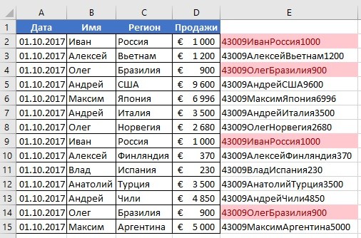
Find matching strings

When this type of comparison is selected, the program finds the strings that match the first and second tables. The strokes in which the values \u200b\u200bin the selected comparison columns (1, 2, 3) are completely coincided with the values \u200b\u200bof the second table columns.

An example of the program in this mode is presented to the right in the picture.

Match table based on selected

In this comparison mode, opposite each row of the first table (selected as the main), the data of the matching line of the second table is copied. In the event that there are no matching lines, the line opposite the main table remains empty.

Comparison of tables in four or more columns

If you lack the program functionality and you need to match the tables in four or more columns, then you can exit the position as follows:

• Create in tables on an empty column.
• In new columns using the formula \u003d Tie Combine the columns that you want to make a comparison.

Thus, you will receive 1 column containing the values \u200b\u200bof several columns. Well, how to match one column you already know.

Perhaps everyone who works with the data in Excel faces the question of how to compare two columns in Excel on coincidence and differences. There are several ways to do it. Let's look at the details each of them.

How to compare two columns in Excel for rows

Comparing the two columns with data, it is often necessary to compare the data in each individual line on the coincidence or difference. We can make such an analysis using a function. Consider how it works on the examples below.

Example 1. How to compare two columns on coincidence and differences in one row

In order to compare the data in each line of two columns in Excel, we will write a simple formula. Insert the formula should be in each line in a nearby column, next to the table in which the main data is posted. By creating a formula for the first line of the table, we can stretch it / copy to the other lines.

In order to check whether the two columns of one line contain the same data, we will need a formula:

\u003d If (A2 \u003d B2; "coincide"; "")

The formula that determines the differences between the two columns in one line will look like this:

\u003d If (A2<>B2; "Do not match"; "")

We can follow the check on the coincidence and the differences between the two columns in one line in the same formula:

\u003d If (a2 \u003d b2; "coincide"; "do not match")

\u003d If (A2<>B2; "Do not match"; "Match up")

An example of the result of calculations may look like this:

In order to compare the data in two columns of one line, with regard to the register, the formula should be used:

\u003d If (coincide (A2, B2); "coincides"; "unique")

How to compare several columns on match in one Excel line

In Excel, it is possible to compare the data in several columns of one row in the following criteria:

• Find rows with the same values \u200b\u200bin all columns of the table;
• Find rows with the same values \u200b\u200bin any two table columns;

Example1. How to find coincidences in one row in several columns of the table

Imagine that our table consists of several columns with data. Our task to find lines in which values \u200b\u200bcoincide in all columns. This will be helped by the Excel functions and. The formula for determining the coincidences will be as follows:

\u003d If (and (a2 \u003d b2; a2 \u003d c2); "coincide"; "")

If there are a lot of columns in our table, it will easily use a function in combination with:

\u003d If (counted ($ A2: $ C2; $ A2) \u003d 3; "coincide"; "")

In the formula as "5" indicates the number of columns of the table for which we created the formula. If your table is more or less in your table, then this value should be equal to the number of columns.

Example 2. How to find coincidences in one row in any two table columns

Imagine that our task is to identify from a table with a few columns those strings in which the data coincides or repeated at least in two columns. This will help us with functions and. We write a formula for a table consisting of three columns with data:

\u003d If (or (a2 \u003d b2; b2 \u003d c2; a2 \u003d c2); "coincide"; "")

In cases where there are too many columns in our table - our formula with a function will be very large, since in its parameters we need to specify the criteria for the coincidence between each column of the table. An easier way, in this case, use the function.

\u003d If (b2: d2; a2) + counted (c2: d2; b2) + (c2 \u003d d2) \u003d 0; "Unique string"; "not a unique string")

\u003d If (counted ($ B: $ B; $ A5) \u003d 0; "There are no coincidences in column B"; "There are coincidences in the column in")

This formula checks the values \u200b\u200bin the column B to coincide with the data of the cells in the column A.

If your table consists of a fixed number of rows, you can specify a clear range in the formula (for example, $ B2: $ B10 ). This will speed up the work of the formula.

How to compare two columns in Excel on coincidence and allocate color

When we are looking for coincidences between the two columns in Excel, we may need to visualize the found coincidences or differences in data, for example, using color isolation. The easiest way to highlight the collarms and differences is to use "Conditional Formatting" in Excel. Consider how to do this in the examples below.

Search and highlighting coincidences in several columns in Excel

In cases where we need to find coincidences in several columns, then for this we need:

• Select columns with data in which you need to calculate the coincidences;
• On the Home tab, on the toolbar, click on the "Conditional Formatting" menu item -\u003e "Code Selection Rules" -\u003e "Repeating Values";
• In the pop-up dialog box, select "Repeat" in the left drop-up list, select repeating values \u200b\u200bin the right drop-down list. Click "OK":
• After that, the column will be highlighted in the selected column:

Search and select color matching strings in Excel

Search for coinciding cells with data in two, several columns and search for the coincidences of whole lines with data is different concepts. Pay attention to the two tables below:

The tables above place the same data. Their difference is that on the example of the left we were looking for coinciding cells, and on the right we found entire repeating lines with the data.

Consider how to find matching lines in the table:

• To the right of the table with the data, we will create auxiliary column in which opposite each row with a data with a simple formula that combines all the values \u200b\u200bof the table string in one cell:

\u003d A2 & B2 & C2 & D2

In the auxiliary column you will see the United Table data:

Now, to determine the coinciding lines in the table, take the following steps:

• Select the area with data in the auxiliary column (in our example it is a range of cells E2: E15 );
• On the Home tab, on the toolbar, click on the "Conditional Formatting" menu item -\u003e "Code Selection Rules" -\u003e "Repeating Values";
• In the pop-up dialog box, select in the left drop-down list "Repeating", in the right drop-down list, select how repeated values \u200b\u200bwill be highlighted. Click "OK":
• After that, duplicate lines will be highlighted in the selected column:

Sometimes you want to view in the Access table only those records that are complied with the records from another table containing fields with the coincident data. For example, you may need to see the records of employees who have treated at least one order to determine which of them deserves encouragement. Or you may need to view the contact details of customers living in one city with an employee to organize a personal meeting.

If you need to compare two ACCESS tables and find the coinciding data, two options are possible.

Create a request that combines fields from each table that contains the appropriate data using an existing link or a combination created for the request. This method is optimal in the speed of returning the results of the query, but does not allow combining fields with different types of data.

Create a query to compare fields in which one field is used as a condition for the other. This method usually requires more time, because when merging the line is excluded from the query results before reading the basic tables, while the conditions apply to the query results after reading these tables. But the field can be used as a condition for comparing fields with different types of data, which cannot be done when using associations.

This article discusses the comparison of two tables to identify the coincidence data and a sample of data that can be used in the examples examples is given.

In this article

Comparison of two tables using associations

To compare the two tables using merges, you need to create a selection request, including both tables. If there is no connection between the tables in the fields containing the necessary data, you need to create associations on them. Associations can be created as much as possible, but each pair of combined fields must contain the data of the same or compatible type.

Suppose you work at the university and want to learn how recent changes in curriculum in mathematics influenced students' assessments. In particular, you are interested in estimating those students who have a form of mathematics. You already have a table containing data on profiling subjects, and a table containing the data on students that are studied. Evaluation data is stored in the "Students" table, and data on profiling items in the Specialization Table. To see how after recent changes in the curriculum, estimates have changed from those who specialize in mathematics, you need to view records from the "Students" table corresponding to the records in the Specialization Table.

Preparation of Data Example

In this example, you create a request that defines how recent changes in the curriculum in mathematics influenced students with the appropriate profiling subject. Use the two tables below: "specializations" and "students". Add them to the database.

Access provides several ways to add these tables a sample database. You can manually enter data, copy each table into the program's spreadsheet (for example, Microsoft Office Excel 2007) and then import sheets in Access or you can insert data in a text editor, such as a notepad and then import data from the resulting text files.

In step-by-step instructions, this section explains how to enter data manually on an empty sheet, as well as how to copy examples of tables in Excel and then import them into Access.

Specialization

Student code		Specialization

Students

Student code		Semester	Syllabus	Subject number	Evaluation

If you are going to enter an example of data in a spreadsheet, you can.

Entering data examples manually

If you are not interested in creating a sheet based on the data example, skip the following partition ("Creating sheets with data examples").

Creating sheets with data examples

Creating sheet database tables based on sheets

Comparison of table samples and search for relevant entries using associations

Now everything is ready for comparing the "Students" and "specialization" tables. Since the connections between the two tables are not defined, you need to create merges the corresponding fields in the request. Tables contain several fields, and you will need to create an association for each pair of shared fields: "student code", "year", as well as a "curriculum" (in the "Student Table") and "specialization" (in the Specialization Table) . In this case, we are only interested in mathematics, so you can limit the results of the query using the field condition.

On the tab Creature Press the button Designer of requests.

In the dialog box Adding a table Double-click the table that contains the necessary records ( Students), and then double-click the table with which it compares it ( Specialization).

Close the dialog box Adding a table.

Drag the field Student code from the table Students in field Student code Tables Specialization. A line will appear in the query form between the two tables, which shows that the union is created. Double-click the line to open the dialog box. Union parameters.

Pay attention to the three options in the dialog box. Union parameters. The default option 1. In some cases, additional lines from one table are required to add to the merge settings. Since you need to find only the coinciding data, leave for merging the value 1. Close the dialog box Union parametersBy pressing the button Cancel.

You need to create two more associations. To do this drag the field Year from the table Students in field Year Tables Specializationand then - field Syllabus from the table Students in field Specialization Tables Specialization.

Table Students Double click Star ( * ) To add all the fields of the table in the request form.

Note: Students. *.

Table Specialization Double-click the field SpecializationTo add it to the blank.

Show column Specialization.

In line Selection condition column Specialization Enter Mat.

On the tab Constructor in a group results Press the button Perform.

Comparison of two tables using the field as a condition

Sometimes it is necessary to compare tables based on fields with matching values, but different types of data. For example, the field in one table may have a numeric data type, and it is necessary to compare it with a field from another table, which has a text data type. Fields containing similar data from different types may appear when saving numbers as text (for example, when importing data from another program). Since it is impossible to create field combining fields with different types of data, you will need to use another way. To compare two fields with different type data, you can use one field as a condition for the other.

Suppose you work at the university and want to learn how recent changes in curriculum in mathematics influenced students' assessments. In particular, you are interested in estimating those students who have a form of mathematics. You already have the "specialization" and "students" tables. Evaluation data is stored in the "Students" table, and data on profiling items in the Specialization Table. To see how the assessments have changed from those who specialize in mathematics, you need to view recordings from the "Students" table, corresponding to the records in the Specialization Table. However, one of the fields you want to use to compare tables, the data type is not like the field with which it is compared.

To compare the two tables using the field as a condition, you need to create a selection request, including both tables. Turn on the field request you want to display, as well as the field corresponding to the field that will be used as a condition. Create a condition for comparing tables. You can create as many conditions as the fields are required for comparison.

To illustrate this method, we use, but in the "Student Code" field, the "specialization" table will change the number of data on text. Since it is impossible to create a combination of two fields with different types of data, we will have to compare two fields "student code" using one field as a condition for the other.

Changing the data type in the "Student Code" field "Specialization"

Open the database in which you saved examples of tables.

IN areas of navigation Click the "specialization" table with the right mouse button and select item. Constructor.

The "specialization" table will open in the constructor mode.

In column Data type Change for field Student code Data type Number on the Text.

Close the "specialization" table. Press the button YesWhen you are prompted to save changes.

Comparison of table examples and search for relevant entries using field condition

Below is shown how to compare the two fields "student code" using the field from the "Students" table as the condition for the field from the Specialization Table. With the help of a keyword Like You can compare two fields, even if they contain different types of data.

On the tab Create in a group Other Press the button Designer of requests.

In the dialog box Adding a table Double-click Table Studentsand then table Specialization.

Close the dialog box Adding a table.

Drag the field Year from the table Students in field Year Tables Specializationand then - field Syllabus from the table Students in field Specialization Tables Specialization. These fields contain the data of the same type, so for their comparison, you can use associations. To compare fields with a single type data, it is recommended to use merges.

Double click Star ( * ) Table StudentsTo add all the fields of the table in the request form.

Note: When using an asterisk to add all fields in the form, only one column is displayed. The name of this column includes the name of the table, followed by the point (.) And asterisk (*). In this example, the column gets the name Students. *.

Table Specialization Double-click the field Student codeTo add it to the blank.

In the query form, uncheck the box in the string Show column Student code. In line Selection condition column Student code Enter Like [Students]. [Student code].

Table Specialization Double-click the field SpecializationTo add it to the blank.

In the query form, uncheck the box in the string Show column Specialization. In line Selection condition Enter Mat.

On the tab Constructor in a group results Press the button Perform.

The request is executed, and evaluations are displayed in mathematics of only those students who have this subject profiling.